6 Section 5 Overview
In Section 5, you will learn about Bayesian statistics through looking at examples from rare disease diagnosis and baseball.
After completing Section 5, you will be able to:
- Apply Bayes’ theorem to calculate the probability of A given B.
- Understand how to use hierarchical models to make better predictions by considering multiple levels of variability.
- Compute a posterior probability using an empirical Bayesian approach.
- Calculate a 95% credible interval from a posterior probability.
6.1 Bayesian Statistics
The textbook for this section is available here.
Key points
- In the urn model, it does not make sense to talk about the probability of \(p\) being greater than a certain value because \(p\) is a fixed value.
- With Bayesian statistics, we assume that \(p\) is in fact random, which allows us to calculate probabilities related to \(p\).
- Hierarchical models describe variability at different levels and incorporate all these levels into a model for estimating \(p\).
6.2 Bayes’ Theorem
The textbook for this section is available here.
Key points
- Bayes’ Theorem states that the probability of event A happening given event B is equal to the probability of both A and B divided by the probability of event B:
\(\mbox{Pr}(A \mid B) = \frac{\mbox{Pr}(B \mid A)\mbox{Pr}(A)}{\mbox{Pr}(B)}\)
- Bayes’ Theorem shows that a test for a very rare disease will have a high percentage of false positives even if the accuracy of the test is high.
Equations: Cystic fibrosis test probabilities
In these probabilities, + represents a positive test, - represents a negative test, \(D = 0\) indicates no disease, and \(D = 1\) indicates the disease is present.
Probability of having the disease given a positive test: \(\mbox{Pr}(D = 1 \mid +)\)
99% test accuracy when disease is present: \(\mbox{Pr}(+ \mid D = 1) = 0.99\)
99% test accuracy when disease is absent: \(\mbox{Pr}(- \mid D = 0) = 0.99\)
Rate of cystic fibrosis: \(\mbox{Pr}(D = 1) = 0.00025\)
Bayes’ theorem can be applied like this:
\(\mbox{Pr}(D = 1 \mid +) = \frac{\mbox{Pr}(+ \mid D = 1)⋅\mbox{Pr}(D = 1)}{\mbox{Pr}(+)}\)
\(\mbox{Pr}(D = 1 \mid +) = \frac{\mbox{Pr}(+ \mid D = 1)⋅\mbox{Pr}(D = 1)}{\mbox{Pr}(+ \mid D=1)⋅\mbox{Pr}(D = 1) + \mbox{Pr}(+ \mid D = 0)⋅\mbox{Pr}(D = 0)}\)
Substituting known values, we obtain:
\(\frac{0.99⋅0.00025}{0.99⋅0.00025 + 0.01⋅0.99975} = 0.02\)
Code: Monte Carlo simulation
prev <- 0.00025    # disease prevalence
N <- 100000    # number of tests
outcome <- sample(c("Disease", "Healthy"), N, replace = TRUE, prob = c(prev, 1-prev))

N_D <- sum(outcome == "Disease")    # number with disease
N_H <- sum(outcome == "Healthy")    # number healthy

# for each person, randomly determine if test is + or -
accuracy <- 0.99
test <- vector("character", N)
test[outcome == "Disease"] <- sample(c("+", "-"), N_D, replace=TRUE, prob = c(accuracy, 1-accuracy))
test[outcome == "Healthy"] <- sample(c("-", "+"), N_H, replace=TRUE, prob = c(accuracy, 1-accuracy))

table(outcome, test)
## test
## outcome - +
## Disease 0 27
## Healthy 99013 9606.3 Bayes in Practice
The textbook for this section is available here.
Key points
- The techniques we have used up until now are referred to as frequentist statistics as they consider only the frequency of outcomes in a dataset and do not include any outside information. Frequentist statistics allow us to compute confidence intervals and p-values.
- Frequentist statistics can have problems when sample sizes are small and when the data are extreme compared to historical results.
- Bayesian statistics allows prior knowledge to modify observed results, which alters our conclusions about event probabilities.
6.4 The Hierarchical Model
The textbook for this section is available here.
Key points
- Hierarchical models use multiple levels of variability to model results. They are hierarchical because values in the lower levels of the model are computed using values from higher levels of the model.
- We model baseball player batting average using a hierarchical model with two levels of variability:
- \(p \sim N(\mu, \tau)\) describes player-to-player variability in natural ability to hit, which has a mean \(\mu\) and standard deviation \(\tau\).
- \(Y \mid p \sim N(p, \sigma)\) describes a player’s observed batting average given their ability \(p\), which has a mean \(p\) and standard deviation \(\sigma = \sqrt{p(1 - p)/N}\). This represents variability due to luck.
- In Bayesian hierarchical models, the first level is called the prior distribution and the second level is called the sampling distribution.
- The posterior distribution allows us to compute the probability distribution of \(p\) given that we have observed data \(Y\).
- By the continuous version of Bayes’ rule, the expected value of the posterior distribution \(p\) given \(Y = y\) is a weighted average between the prior mean \(\mu\) and the observed data \(Y\):
\(\mbox{E}(p \mid y) = B\mu + (1 - B)Y\) where \(B = \frac{\sigma^2}{\sigma^2 + \tau^2}\)
- The standard error of the posterior distribution \(\mbox{SE}(p\mid Y)^2\) is \(\frac{1}{{1/\sigma^2} + {1/\tau^2}}\). Note that you will need to take the square root of both sides to solve for the standard error.
- This Bayesian approach is also known as shrinking. When \(\sigma\) is large, \(B\) is close to 1 and our prediction of \(p\) shrinks towards the mean (\(\mu\)). When \(\sigma\) is small, \(B\) is close to 0 and our prediction of \(p\) is more weighted towards the observed data \(Y\).
6.5 Assessment - Bayesian Statistics
- In 1999 in England Sally Clark was found guilty of the murder of two of her sons.
Both infants were found dead in the morning, one in 1996 and another in 1998, and she claimed the cause of death was sudden infant death syndrome (SIDS). No evidence of physical harm was found on the two infants so the main piece of evidence against her was the testimony of Professor Sir Roy Meadow, who testified that the chances of two infants dying of SIDS was 1 in 73 million. He arrived at this figure by finding that the rate of SIDS was 1 in 8,500 and then calculating that the chance of two SIDS cases was \(8,500 × 8,500 \approx \text{73 million}\).
Based on what we’ve learned throughout this course, which statement best describes a potential flaw in Sir Meadow’s reasoning?
- A. Sir Meadow assumed the second death was independent of the first son being affected, thereby ignoring possible genetic causes.
- B. There is no flaw. The multiplicative rule always applies in this way: \(\mbox{Pr}(\text{A and B}) = \mbox{Pr}(A)\mbox{Pr}(B)\)
- C. Sir Meadow should have added the probabilities: \(\mbox{Pr}(\text{A and B}) = \mbox{Pr}(A) + \mbox{Pr}(B)\)
- D. The rate of SIDS is too low to perform these types of statistics.
- Let’s assume that there is in fact a genetic component to SIDS and the the probability of \(\mbox{Pr}(\text{second case of SIDS} \mid \text{first case of SIDS}) = 1/100\), is much higher than 1 in 8,500.
What is the probability of both of Sally Clark’s sons dying of SIDS?
# Define `Pr_1` as the probability of the first son dying of SIDS
Pr_1 <- 1/8500

# Define `Pr_2` as the probability of the second son dying of SIDS
Pr_2 <- 1/100

# Calculate the probability of both sons dying of SIDS. Print this value to the console.
Pr_1 * Pr_2
## [1] 1.176471e-06- Many press reports stated that the expert claimed the probability of Sally Clark being innocent as 1 in 73 million.
Perhaps the jury and judge also interpreted the testimony this way. This probability can be written like this:
\(\mbox{Pr}(\text{mother is a murderer} \mid \text{two children found dead with no evidence of harm})\)
Bayes’ rule tells us this probability is equal to:
- A. \(\frac{\mbox{Pr}(\text{two children found dead with no evidence of harm})\mbox{Pr}(\text{mother is a murderer})}{\mbox{Pr}(\text{two children found dead with no evidence of harm})}\)
- B. \(\mbox{Pr}(\text{two children found dead with no evidence of harm})\mbox{Pr}(\text{mother is a murderer})\)
- C. \(\frac{\mbox{Pr}(\text{two children found dead with no evidence of harm} \mid \text{mother is a murderer})\mbox{Pr}(\text{mother is a murderer})}{\mbox{Pr}(\text{two children found dead with no evidence of harm})}\)
- D. 1/8500
- Assume that the probability of a murderer finding a way to kill her two children without leaving evidence of physical harm is:
\(\mbox{Pr}(\text{two children found dead with no evidence of harm} \mid \text{mother is a murderer}) = 0.50\)
Assume that the murder rate among mothers is 1 in 1,000,000.
\(\mbox{Pr}(\text{mother is a murderer}) = 1/1,000,000\)
According to Bayes’ rule, what is the probability of:
\(\mbox{Pr}(\text{mother is a murderer} \mid \text{two children found dead with no evidence of harm})\)
# Define `Pr_1` as the probability of the first son dying of SIDS
Pr_1 <- 1/8500

# Define `Pr_2` as the probability of the second son dying of SIDS
Pr_2 <- 1/100

# Define `Pr_B` as the probability of both sons dying of SIDS
Pr_B <- Pr_1*Pr_2

# Define Pr_A as the rate of mothers that are murderers
Pr_A <- 1/1000000

# Define Pr_BA as the probability that two children die without evidence of harm, given that their mother is a murderer
Pr_BA <- 0.50

# Define Pr_AB as the probability that a mother is a murderer, given that her two children died with no evidence of physical harm. Print this value to the console.
Pr_AB <- (Pr_BA * Pr_A)/Pr_B
Pr_AB
## [1] 0.425- After Sally Clark was found guilty, the Royal Statistical Society issued a statement saying that there was “no statistical basis” for the expert’s claim.
They expressed concern at the “misuse of statistics in the courts”. Eventually, Sally Clark was acquitted in June 2003.
In addition to misusing the multiplicative rule as we saw earlier, what else did Sir Meadow miss?
- A. He made an arithmetic error in forgetting to divide by the rate of SIDS in siblings.
- B. He did not take into account how rare it is for a mother to murder her children.
- C. He mixed up the numerator and denominator of Bayes’ rule.
- D. He did not take into account murder rates in the population.
- Florida is one of the most closely watched states in the U.S. election because it has many electoral votes and the election is generally close.
Create a table with the poll spread results from Florida taken during the last days before the election using the sample code.
The CLT tells us that the average of these spreads is approximately normal. Calculate a spread average and provide an estimate of the standard error.
# Create an object `polls` that contains the spread of predictions for each candidate in Florida during the last polling days
polls <- polls_us_election_2016 %>%
  filter(state == "Florida" & enddate >= "2016-11-04" ) %>%
  mutate(spread = rawpoll_clinton/100 - rawpoll_trump/100)

# Examine the `polls` object using the `head` function
head(polls)
## state startdate enddate pollster grade samplesize population rawpoll_clinton rawpoll_trump rawpoll_johnson rawpoll_mcmullin adjpoll_clinton
## 1 Florida 2016-11-03 2016-11-06 Quinnipiac University A- 884 lv 46.00 45.00 2.00 NA 46.44315
## 2 Florida 2016-11-02 2016-11-04 YouGov B 1188 rv 45.00 45.00 NA NA 47.07455
## 3 Florida 2016-11-01 2016-11-07 SurveyMonkey C- 4092 lv 47.00 45.00 4.00 NA 45.59190
## 4 Florida 2016-11-06 2016-11-06 Trafalgar Group C 1100 lv 46.13 49.72 2.43 NA 45.75904
## 5 Florida 2016-11-05 2016-11-06 Opinion Savvy/InsiderAdvantage C- 843 lv 48.40 46.40 3.00 NA 47.37976
## 6 Florida 2016-11-02 2016-11-06 Rasmussen Reports/Pulse Opinion Research C+ 525 lv 47.00 45.00 2.00 NA 47.55885
## adjpoll_trump adjpoll_johnson adjpoll_mcmullin spread
## 1 43.93999 2.098310 NA 0.0100
## 2 46.99468 NA NA 0.0000
## 3 44.32744 1.692430 NA 0.0200
## 4 46.82230 3.495849 NA -0.0359
## 5 45.68637 2.721857 NA 0.0200
## 6 45.13673 2.418502 NA 0.0200# Create an object called `results` that has two columns containing the average spread (`avg`) and the standard error (`se`). Print the results to the console.
results <- polls %>% summarize(avg = mean(spread), se = sd(spread)/sqrt(n()))
results## avg se
## 1 0.004154545 0.007218692- Assume a Bayesian model sets the prior distribution for Florida’s election night spread \(d\) to be normal with expected value \(\mu\) and standard deviation \(\tau\).
What are the interpretations of \(\mu\) and \(\tau\)?
- A. \(\mu\) and \(\tau\) are arbitrary numbers that let us make probability statements about \(d\).
- B. \(\mu\) and \(\tau\) summarize what we would predict for Florida before seeing any polls.
- C. \(\mu\) and \(\tau\) summarize what we want to be true. We therefore set \(\mu\) at 0.10 and \(\tau\) at 0.01.
- D. The choice of prior has no effect on the Bayesian analysis.
- The CLT tells us that our estimate of the spread \(\hat{d}\) has a normal distribution with expected value \(d\) and standard deviation \(\sigma\), which we calculated in a previous exercise.
Use the formulas for the posterior distribution to calculate the expected value of the posterior distribution if we set \(\mu = 0\) and \(\tau = 0.01\).
# The results` object has already been loaded. Examine the values stored: `avg` and `se` of the spread
results
## avg se
## 1 0.004154545 0.007218692# Define `mu` and `tau`
mu <- 0
tau <- 0.01
# Define a variable called `sigma` that contains the standard error in the object `results`
sigma <- results$se
# Define a variable called `Y` that contains the average in the object `results`
Y <- results$avg
# Define a variable `B` using `sigma` and `tau`. Print this value to the console.
B <- sigma^2/(sigma^2+tau^2)
# Calculate the expected value of the posterior distribution
EV <- B*mu + (1-B)*Y
EV## [1] 0.002731286- Compute the standard error of the posterior distribution.
# Here are the variables we have defined
mu <- 0
tau <- 0.01
sigma <- results$se
Y <- results$avg
B <- sigma^2 / (sigma^2 + tau^2)

# Compute the standard error of the posterior distribution. Print this value to the console.
SE <- sqrt(1/((1/sigma^2)+(1/tau^2)))
SE
## [1] 0.005853024- Using the fact that the posterior distribution is normal, create an interval that has a 95% of occurring centered at the posterior expected value.
Note that we call these credible intervals.
# Here are the variables we have defined in previous exercises
mu <- 0
tau <- 0.01
sigma <- results$se
Y <- results$avg
B <- sigma^2 / (sigma^2 + tau^2)
se <- sqrt( 1/ (1/sigma^2 + 1/tau^2))

# Construct the 95% credible interval. Save the lower and then the upper confidence interval to a variable called `ci`.
ev <- B*mu + (1-B)*Y
ci <- c(ev - qnorm(0.975) * se, ev + qnorm(0.975) * se)
ci
## [1] -0.008740432 0.014203003- According to this analysis, what was the probability that Trump wins Florida?
# Assign the expected value of the posterior distribution to the variable `exp_value`
exp_value <- B*mu + (1-B)*Y
# Assign the standard error of the posterior distribution to the variable `se`
se <- sqrt( 1/ (1/sigma^2 + 1/tau^2))
# Using the `pnorm` function, calculate the probability that the actual spread was less than 0 (in Trump's favor). Print this value to the console.
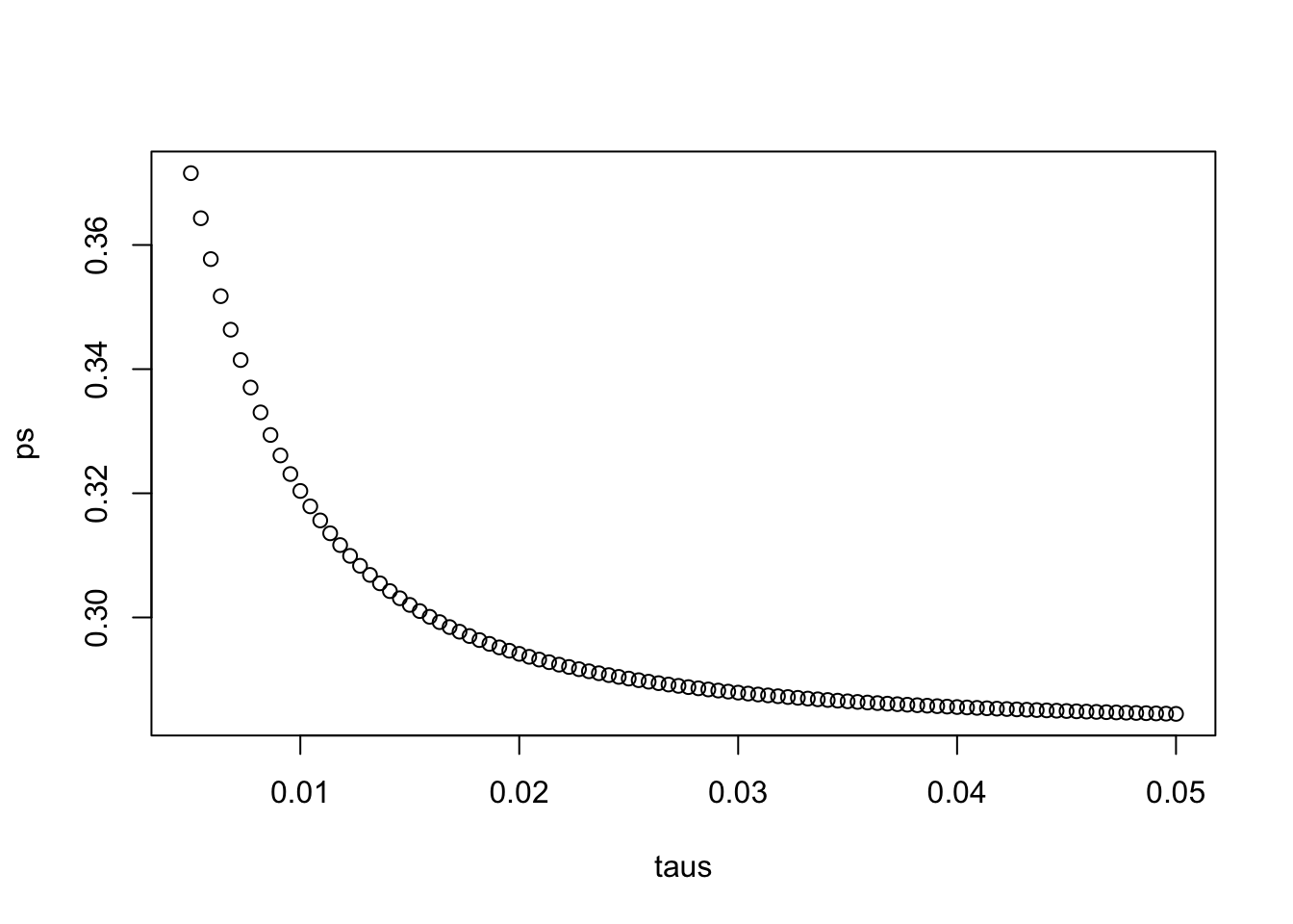
pnorm(0, exp_value, se)## [1] 0.3203769- We had set the prior variance \(\tau\) to 0.01, reflecting that these races are often close.
Change the prior variance to include values ranging from 0.005 to 0.05 and observe how the probability of Trump winning Florida changes by making a plot.
# Define the variables from previous exercises
mu <- 0
sigma <- results$se
Y <- results$avg

# Define a variable `taus` as different values of tau
taus <- seq(0.005, 0.05, len = 100)

# Create a function called `p_calc` that generates `B` and calculates the probability of the spread being less than 0
p_calc <- function(tau) {
    B <- sigma^2 / (sigma^2 + tau^2)
    ev <- B*mu + (1-B)*Y
    se <- sqrt(1 / (1/sigma^2 + 1/tau^2))
    pnorm(0,ev,se)
}

# Create a vector called `ps` by applying the function `p_calc` across values in `taus`
ps <- p_calc(taus)

# Plot `taus` on the x-axis and `ps` on the y-axis
plot(taus, ps)