4 Section 3 - Linear Regression for Prediction, Smoothing, and Working with Matrices Overview

In the Linear Regression for Prediction, Smoothing, and Working with Matrices Overview section, you will learn why linear regression is a useful baseline approach but is often insufficiently flexible for more complex analyses, how to smooth noisy data, and how to use matrices for machine learning.

After completing this section, you will be able to:

• Use linear regression for prediction as a baseline approach.
• Use logistic regression for categorical data.
• Detect trends in noisy data using smoothing (also known as curve fitting or low pass filtering).
• Convert predictors to matrices and outcomes to vectors when all predictors are numeric (or can be converted to numerics in a meaningful way).
• Perform basic matrix algebra calculations.

This section has three parts: linear regression for prediction, smoothing, and working with matrices.

4.1 Linear Regression for Prediction

There is a link to the relevant section of the textbook: Linear regression for prediction

Key points

• Linear regression can be considered a machine learning algorithm. Although it can be too rigid to be useful, it works rather well for some challenges. It also serves as a baseline approach: if you can’t beat it with a more complex approach, you probably want to stick to linear regression.

Code

Note: the seed was not set before createDataPartition so your results may be different.

if(!require(HistData)) install.packages("HistData")

## Loading required package: HistData

library(HistData)

galton_heights <- GaltonFamilies %>%
  filter(childNum == 1 & gender == "male") %>%
  dplyr::select(father, childHeight) %>%
  rename(son = childHeight)

y <- galton_heights$son
test_index <- createDataPartition(y, times = 1, p = 0.5, list = FALSE)

train_set <- galton_heights %>% slice(-test_index)
test_set <- galton_heights %>% slice(test_index)

avg <- mean(train_set$son)
avg

## [1] 70.50114

mean((avg - test_set$son)^2)

## [1] 6.034931

# fit linear regression model
fit <- lm(son ~ father, data = train_set)
fit$coef

## (Intercept)      father 
##  34.8934373   0.5170499

y_hat <- fit$coef[1] + fit$coef[2]*test_set$father
mean((y_hat - test_set$son)^2)

## [1] 4.632629

4.2 Predict Function

There is a link to the relevant section of the textbook: Predict function

Key points

• The predict() function takes a fitted object from functions such as lm() or glm() and a data frame with the new predictors for which to predict. We can use predict like this:

y_hat <- predict(fit, test_set)

• predict() is a generic function in R that calls other functions depending on what kind of object it receives. To learn about the specifics, you can read the help files using code like this:

?predict.lm    # or ?predict.glm

Code

y_hat <- predict(fit, test_set)
mean((y_hat - test_set$son)^2)

## [1] 4.632629

# read help files
?predict.lm
?predict.glm

4.3 Comprehension Check - Linear Regression

1. Create a data set using the following code:

# set.seed(1) # if using R 3.5 or earlier
set.seed(1, sample.kind="Rounding") # if using R 3.6 or later

## Warning in set.seed(1, sample.kind = "Rounding"): non-uniform 'Rounding' sampler used

n <- 100
Sigma <- 9*matrix(c(1.0, 0.5, 0.5, 1.0), 2, 2)
dat <- MASS::mvrnorm(n = 100, c(69, 69), Sigma) %>%
      data.frame() %>% setNames(c("x", "y"))

We will build 100 linear models using the data above and calculate the mean and standard deviation of the combined models. First, set the seed to 1 again (make sure to use sample.kind="Rounding" if your R is version 3.6 or later). Then, within a replicate() loop, (1) partition the dataset into test and training sets with p = 0.5 and using dat$y to generate your indices, (2) train a linear model predicting y from x, (3) generate predictions on the test set, and (4) calculate the RMSE of that model. Then, report the mean and standard deviation (SD) of the RMSEs from all 100 models.

Report all answers to at least 3 significant digits.

# set.seed(1) # if using R 3.5 or earlier
set.seed(1, sample.kind="Rounding") # if using R 3.6 or later

## Warning in set.seed(1, sample.kind = "Rounding"): non-uniform 'Rounding' sampler used

rmse <- replicate(100, {
    test_index <- createDataPartition(dat$y, times = 1, p = 0.5, list = FALSE)
    train_set <- dat %>% slice(-test_index)
    test_set <- dat %>% slice(test_index)
    fit <- lm(y ~ x, data = train_set)
    y_hat <- predict(fit, newdata = test_set)
    sqrt(mean((y_hat-test_set$y)^2))
})

mean(rmse)

## [1] 2.488661

sd(rmse)

## [1] 0.1243952

2. Now we will repeat the exercise above but using larger datasets. Write a function that takes a size n, then (1) builds a dataset using the code provided at the top of Q1 but with n observations instead of 100 and without the set.seed(1), (2) runs the replicate() loop that you wrote to answer Q1, which builds 100 linear models and returns a vector of RMSEs, and (3) calculates the mean and standard deviation of the 100 RMSEs.

Set the seed to 1 (if using R 3.6 or later, use the argument sample.kind="Rounding") and then use sapply() or map() to apply your new function to n <- c(100, 500, 1000, 5000, 10000).

Hint: You only need to set the seed once before running your function; do not set a seed within your function. Also be sure to use sapply() or map() as you will get different answers running the simulations individually due to setting the seed.

# set.seed(1) # if R 3.5 or earlier
set.seed(1, sample.kind="Rounding") # if R 3.6 or later

## Warning in set.seed(1, sample.kind = "Rounding"): non-uniform 'Rounding' sampler used

n <- c(100, 500, 1000, 5000, 10000)
res <- sapply(n, function(n){
    Sigma <- 9*matrix(c(1.0, 0.5, 0.5, 1.0), 2, 2)
    dat <- MASS::mvrnorm(n, c(69, 69), Sigma) %>%
        data.frame() %>% setNames(c("x", "y"))
    rmse <- replicate(100, {
        test_index <- createDataPartition(dat$y, times = 1, p = 0.5, list = FALSE)
        train_set <- dat %>% slice(-test_index)
        test_set <- dat %>% slice(test_index)
        fit <- lm(y ~ x, data = train_set)
        y_hat <- predict(fit, newdata = test_set)
        sqrt(mean((y_hat-test_set$y)^2))
    })
    c(avg = mean(rmse), sd = sd(rmse))
})

res

##          [,1]       [,2]       [,3]       [,4]       [,5]
## avg 2.4977540 2.72095125 2.55554451 2.62482800 2.61844227
## sd  0.1180821 0.08002108 0.04560258 0.02309673 0.01689205

3. What happens to the RMSE as the size of the dataset becomes larger?

• A. On average, the RMSE does not change much as n gets larger, but the variability of the RMSE decreases.
• B. Because of the law of large numbers the RMSE decreases; more data means more precise estimates.
• C. n = 10000 is not sufficiently large. To see a decrease in the RMSE we would need to make it larger.
• D. The RMSE is not a random variable.

4. Now repeat the exercise from Q1, this time making the correlation between x and y larger, as in the following code:

# set.seed(1) # if using R 3.5 or earlier
set.seed(1, sample.kind="Rounding") # if using R 3.6 or later

## Warning in set.seed(1, sample.kind = "Rounding"): non-uniform 'Rounding' sampler used

n <- 100
Sigma <- 9*matrix(c(1.0, 0.95, 0.95, 1.0), 2, 2)
dat <- MASS::mvrnorm(n = 100, c(69, 69), Sigma) %>%
    data.frame() %>% setNames(c("x", "y"))

Note what happens to RMSE - set the seed to 1 as before.

# set.seed(1) # if using R 3.5 or earlier
set.seed(1, sample.kind="Rounding") # if using R 3.6 or later

## Warning in set.seed(1, sample.kind = "Rounding"): non-uniform 'Rounding' sampler used

rmse <- replicate(100, {
    test_index <- createDataPartition(dat$y, times = 1, p = 0.5, list = FALSE)
    train_set <- dat %>% slice(-test_index)
    test_set <- dat %>% slice(test_index)
    fit <- lm(y ~ x, data = train_set)
    y_hat <- predict(fit, newdata = test_set)
    sqrt(mean((y_hat-test_set$y)^2))
})

mean(rmse)

## [1] 0.9099808

sd(rmse)

## [1] 0.06244347

5. Which of the following best explains why the RMSE in question 4 is so much lower than the RMSE in question 1?

• A. It is just luck. If we do it again, it will be larger.
• B. The central limit theorem tells us that the RMSE is normal.
• C. When we increase the correlation between x and y, x has more predictive power and thus provides a better estimate of y.
• D. These are both examples of regression so the RMSE has to be the same.

6. Create a data set using the following code.

# set.seed(1) # if using R 3.5 or earlier
set.seed(1, sample.kind="Rounding") # if using R 3.6 or later

## Warning in set.seed(1, sample.kind = "Rounding"): non-uniform 'Rounding' sampler used

Sigma <- matrix(c(1.0, 0.75, 0.75, 0.75, 1.0, 0.25, 0.75, 0.25, 1.0), 3, 3)
dat <- MASS::mvrnorm(n = 100, c(0, 0, 0), Sigma) %>%
    data.frame() %>% setNames(c("y", "x_1", "x_2"))

Note that y is correlated with both x_1 and x_2 but the two predictors are independent of each other, as seen by cor(dat).

Set the seed to 1, then use the caret package to partition into test and training sets with p = 0.5. Compare the RMSE when using just x_1, just x_2 and both x_1 and x_2. Train a single linear model for each (not 100 like in the previous questions).

Which of the three models performs the best (has the lowest RMSE)?

# set.seed(1) # if using R 3.5 or earlier
set.seed(1, sample.kind="Rounding") # if using R 3.6 or later

## Warning in set.seed(1, sample.kind = "Rounding"): non-uniform 'Rounding' sampler used

test_index <- createDataPartition(dat$y, times = 1, p = 0.5, list = FALSE)
train_set <- dat %>% slice(-test_index)
test_set <- dat %>% slice(test_index)

fit <- lm(y ~ x_1, data = train_set)
y_hat <- predict(fit, newdata = test_set)
sqrt(mean((y_hat-test_set$y)^2))

## [1] 0.600666

fit <- lm(y ~ x_2, data = train_set)
y_hat <- predict(fit, newdata = test_set)
sqrt(mean((y_hat-test_set$y)^2))

## [1] 0.630699

fit <- lm(y ~ x_1 + x_2, data = train_set)
y_hat <- predict(fit, newdata = test_set)
sqrt(mean((y_hat-test_set$y)^2))

## [1] 0.3070962

• A. x_1
• B. x_2
• C. x_1 and x_2

7. Report the lowest RMSE of the three models tested in Q6.

fit <- lm(y ~ x_1 + x_2, data = train_set)
y_hat <- predict(fit, newdata = test_set)
sqrt(mean((y_hat-test_set$y)^2))

## [1] 0.3070962

8. Repeat the exercise from Q6 but now create an example in which x_1 and x_2 are highly correlated.

# set.seed(1) # if using R 3.5 or earlier
set.seed(1, sample.kind="Rounding") # if using R 3.6 or later

## Warning in set.seed(1, sample.kind = "Rounding"): non-uniform 'Rounding' sampler used

Sigma <- matrix(c(1.0, 0.75, 0.75, 0.75, 1.0, 0.95, 0.75, 0.95, 1.0), 3, 3)
dat <- MASS::mvrnorm(n = 100, c(0, 0, 0), Sigma) %>%
    data.frame() %>% setNames(c("y", "x_1", "x_2"))

Set the seed to 1, then use the caret package to partition into a test and training set of equal size. Compare the RMSE when using just x_1, just x_2, and both x_1 and x_2.

Compare the results from Q6 and Q8. What can you conclude?

# set.seed(1) # if using R 3.5 or earlier
set.seed(1, sample.kind="Rounding") # if using R 3.6 or later

## Warning in set.seed(1, sample.kind = "Rounding"): non-uniform 'Rounding' sampler used

test_index <- createDataPartition(dat$y, times = 1, p = 0.5, list = FALSE)
train_set <- dat %>% slice(-test_index)
test_set <- dat %>% slice(test_index)

fit <- lm(y ~ x_1, data = train_set)
y_hat <- predict(fit, newdata = test_set)
sqrt(mean((y_hat-test_set$y)^2))

## [1] 0.6592608

fit <- lm(y ~ x_2, data = train_set)
y_hat <- predict(fit, newdata = test_set)
sqrt(mean((y_hat-test_set$y)^2))

## [1] 0.640081

fit <- lm(y ~ x_1 + x_2, data = train_set)
y_hat <- predict(fit, newdata = test_set)
sqrt(mean((y_hat-test_set$y)^2))

## [1] 0.6597865

• A. Unless we include all predictors we have no predictive power.
• B. Adding extra predictors improves RMSE regardless of whether the added predictors are correlated with other predictors or not.
• C. Adding extra predictors results in over fitting.
• D. Adding extra predictors can improve RMSE substantially, but not when the added predictors are highly correlated with other predictors.

4.4 Regression for a Categorical Outcome

There is a link to the relevant section of the textbook: Regression for a categorical outcome

Key points

• The regression approach can be extended to categorical data. For example, we can try regression to estimate the conditional probability:

\(p(x)=Pr(Y=1|X=x)=\beta_{0}+\beta_{1}x\)

• Once we have estimates \(\beta_0\) and \(\beta_1\), we can obtain an actual prediction \(p(x)\). Then we can define a specific decision rule to form a prediction.

Code

data("heights")
y <- heights$height

set.seed(2) #if you are using R 3.5 or earlier
set.seed(2, sample.kind = "Rounding") #if you are using R 3.6 or later

## Warning in set.seed(2, sample.kind = "Rounding"): non-uniform 'Rounding' sampler used

test_index <- createDataPartition(y, times = 1, p = 0.5, list = FALSE)
train_set <- heights %>% slice(-test_index)
test_set <- heights %>% slice(test_index)

train_set %>% 
  filter(round(height)==66) %>%
  summarize(y_hat = mean(sex=="Female"))

##       y_hat
## 1 0.2424242

heights %>% 
  mutate(x = round(height)) %>%
  group_by(x) %>%
  filter(n() >= 10) %>%
  summarize(prop = mean(sex == "Female")) %>%
  ggplot(aes(x, prop)) +
  geom_point()

## `summarise()` ungrouping output (override with `.groups` argument)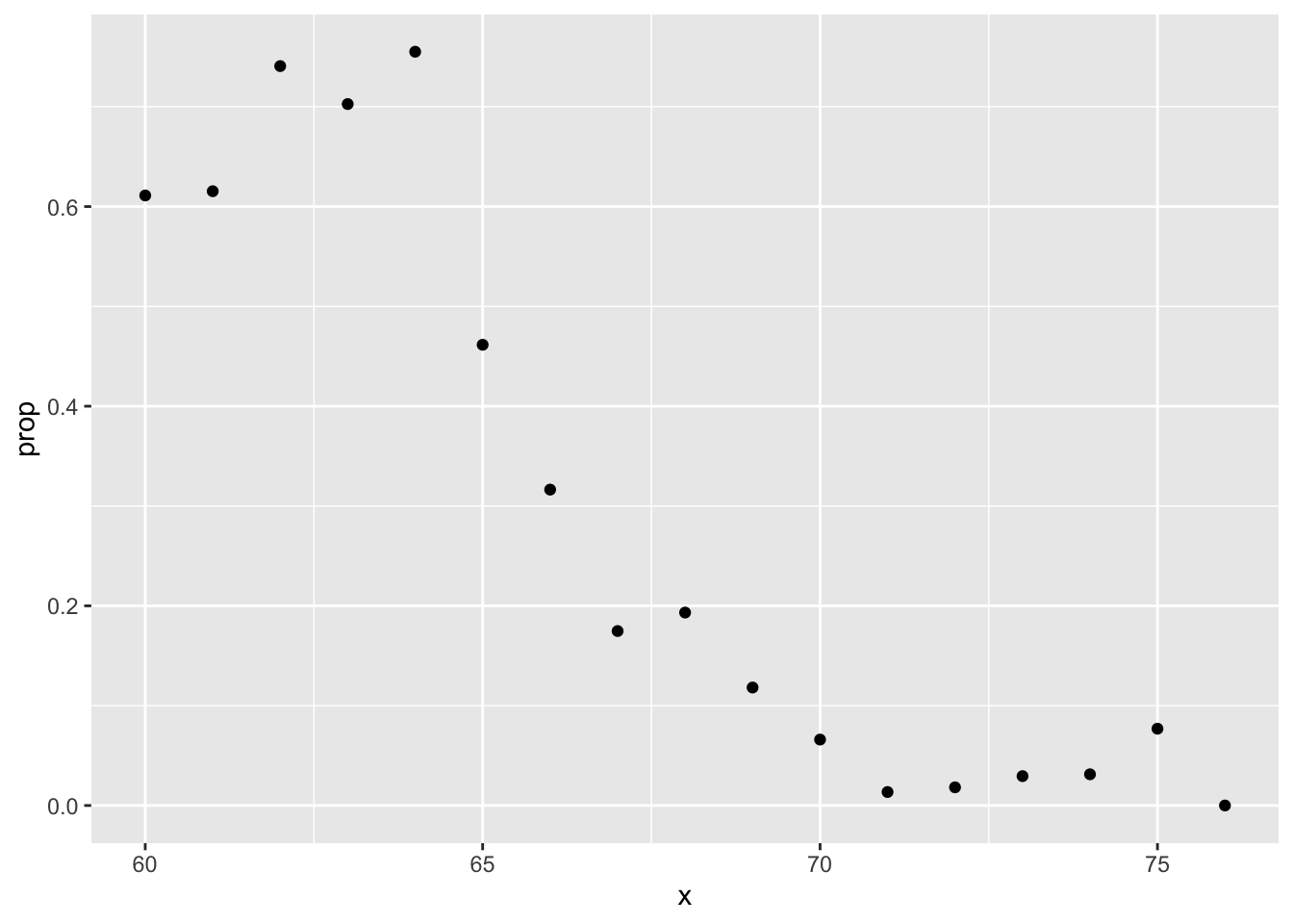

lm_fit <- mutate(train_set, y = as.numeric(sex == "Female")) %>% lm(y ~ height, data = .)
p_hat <- predict(lm_fit, test_set)
y_hat <- ifelse(p_hat > 0.5, "Female", "Male") %>% factor()
confusionMatrix(y_hat, test_set$sex)$overall["Accuracy"]

##  Accuracy 
## 0.7851711

4.5 Logistic Regression

There is a link to the relevant section of the textbook: Logistic regression

Key points

• Logistic regression is an extension of linear regression that assures that the estimate of conditional probability \(Pr(Y=1|X=x)\) is between 0 and 1. This approach makes use of the logistic transformation:

\(g(p)=log\frac{p}{1-p}\)

• With logistic regression, we model the conditional probability directly with:

\(g\{Pr(Y=1|X=x)\}=\beta_{0}+\beta_{1}x\)

• Note that with this model, we can no longer use least squares. Instead we compute the maximum likelihood estimate (MLE).
• In R, we can fit the logistic regression model with the function glm() (generalized linear models). If we want to compute the conditional probabilities, we want type="response" since the default is to return the logistic transformed values.

Code

heights %>% 
  mutate(x = round(height)) %>%
  group_by(x) %>%
  filter(n() >= 10) %>%
  summarize(prop = mean(sex == "Female")) %>%
  ggplot(aes(x, prop)) +
  geom_point() + 
  geom_abline(intercept = lm_fit$coef[1], slope = lm_fit$coef[2])

## `summarise()` ungrouping output (override with `.groups` argument)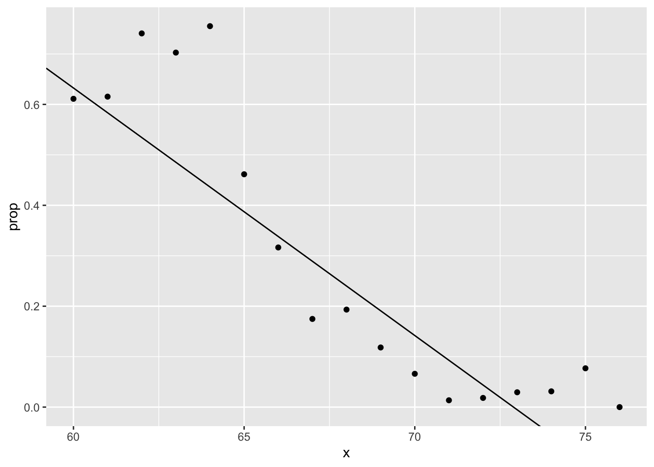

range(p_hat)

## [1] -0.397868  1.123309

# fit logistic regression model
glm_fit <- train_set %>% 
  mutate(y = as.numeric(sex == "Female")) %>%
  glm(y ~ height, data=., family = "binomial")

p_hat_logit <- predict(glm_fit, newdata = test_set, type = "response")

tmp <- heights %>% 
  mutate(x = round(height)) %>%
  group_by(x) %>%
  filter(n() >= 10) %>%
  summarize(prop = mean(sex == "Female")) 

## `summarise()` ungrouping output (override with `.groups` argument)

logistic_curve <- data.frame(x = seq(min(tmp$x), max(tmp$x))) %>%
  mutate(p_hat = plogis(glm_fit$coef[1] + glm_fit$coef[2]*x))
tmp %>% 
  ggplot(aes(x, prop)) +
  geom_point() +
  geom_line(data = logistic_curve, mapping = aes(x, p_hat), lty = 2)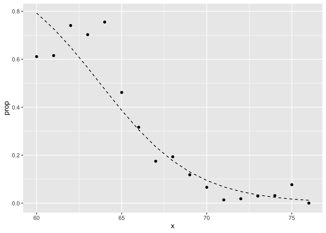

y_hat_logit <- ifelse(p_hat_logit > 0.5, "Female", "Male") %>% factor
confusionMatrix(y_hat_logit, test_set$sex)$overall[["Accuracy"]]

## [1] 0.7984791

4.6 Case Study: 2 or 7

There is a link to the relevant section of the textbook: Case study: 2 or 7

Key points

• In this case study we apply logistic regression to classify whether a digit is two or seven. We are interested in estimating a conditional probability that depends on two variables:

\(g\{p(x_{1},x_{2}\}=g\{Pr(Y=1|X_{1}=x_{1}, X_{2}=x_{2})\} = \beta_{0}+\beta_{1}x_{1}+\beta_{2}x_{2}\)

• Through this case, we know that logistic regression forces our estimates to be a plane and our boundary to be a line. This implies that a logistic regression approach has no chance of capturing the non-linear nature of the true \(p(x_{1}, x_{2})\). Therefore, we need other more flexible methods that permit other shapes.

Code

mnist <- read_mnist()
is <- mnist_27$index_train[c(which.min(mnist_27$train$x_1), which.max(mnist_27$train$x_1))]
titles <- c("smallest","largest")
tmp <- lapply(1:2, function(i){
    expand.grid(Row=1:28, Column=1:28) %>%
        mutate(label=titles[i],
               value = mnist$train$images[is[i],])
})
tmp <- Reduce(rbind, tmp)
tmp %>% ggplot(aes(Row, Column, fill=value)) +
    geom_raster() +
    scale_y_reverse() +
    scale_fill_gradient(low="white", high="black") +
    facet_grid(.~label) +
    geom_vline(xintercept = 14.5) +
    geom_hline(yintercept = 14.5)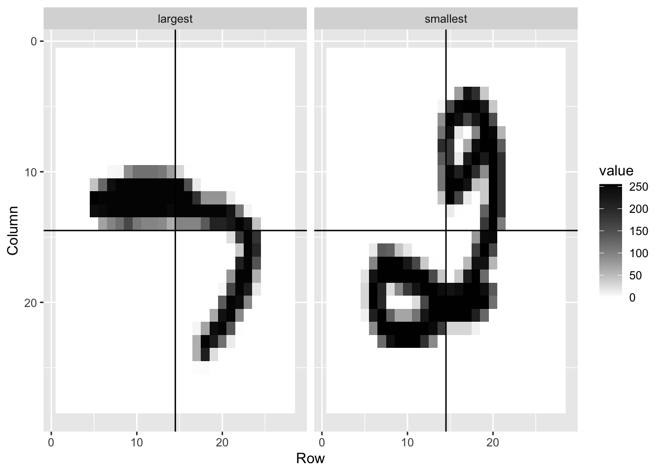

data("mnist_27")
mnist_27$train %>% ggplot(aes(x_1, x_2, color = y)) + geom_point()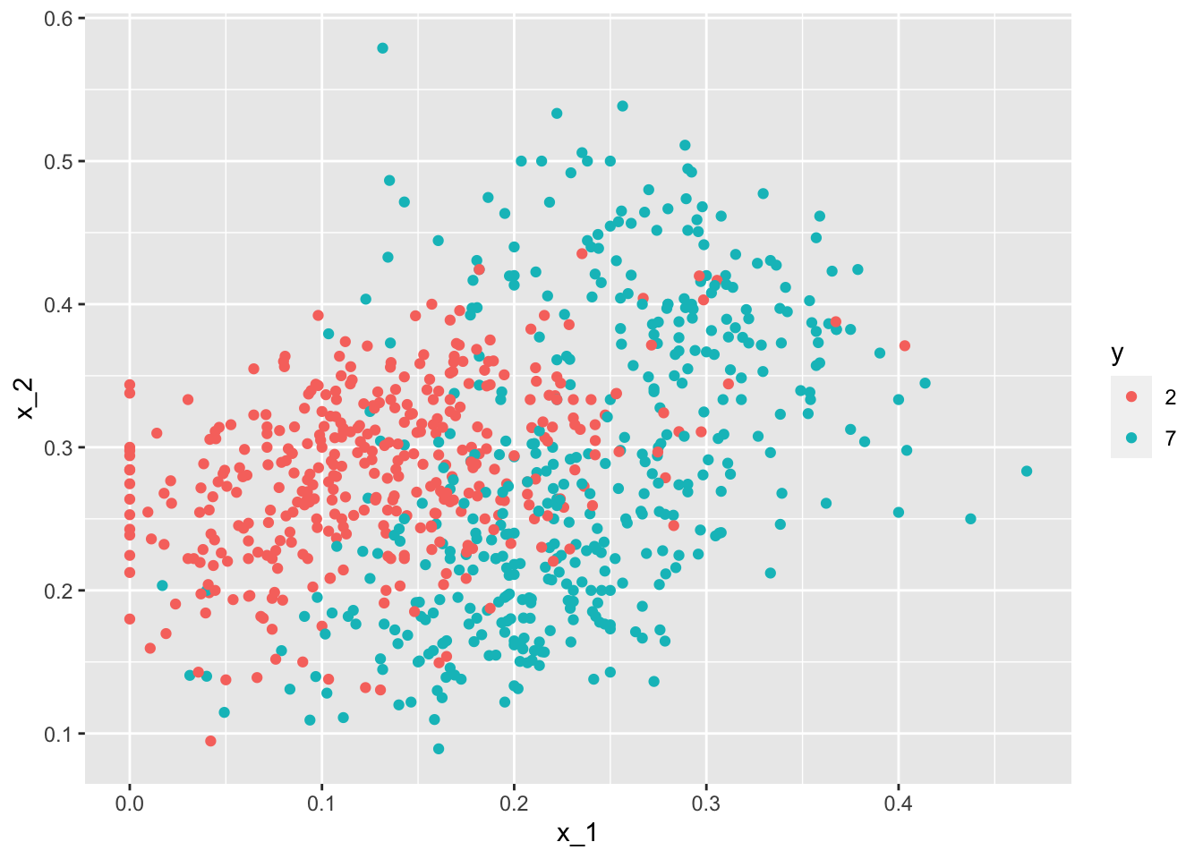

is <- mnist_27$index_train[c(which.min(mnist_27$train$x_2), which.max(mnist_27$train$x_2))]
titles <- c("smallest","largest")
tmp <- lapply(1:2, function(i){
    expand.grid(Row=1:28, Column=1:28) %>%
        mutate(label=titles[i],
               value = mnist$train$images[is[i],])
})
tmp <- Reduce(rbind, tmp)
tmp %>% ggplot(aes(Row, Column, fill=value)) +
    geom_raster() +
    scale_y_reverse() +
    scale_fill_gradient(low="white", high="black") +
    facet_grid(.~label) +
    geom_vline(xintercept = 14.5) +
    geom_hline(yintercept = 14.5)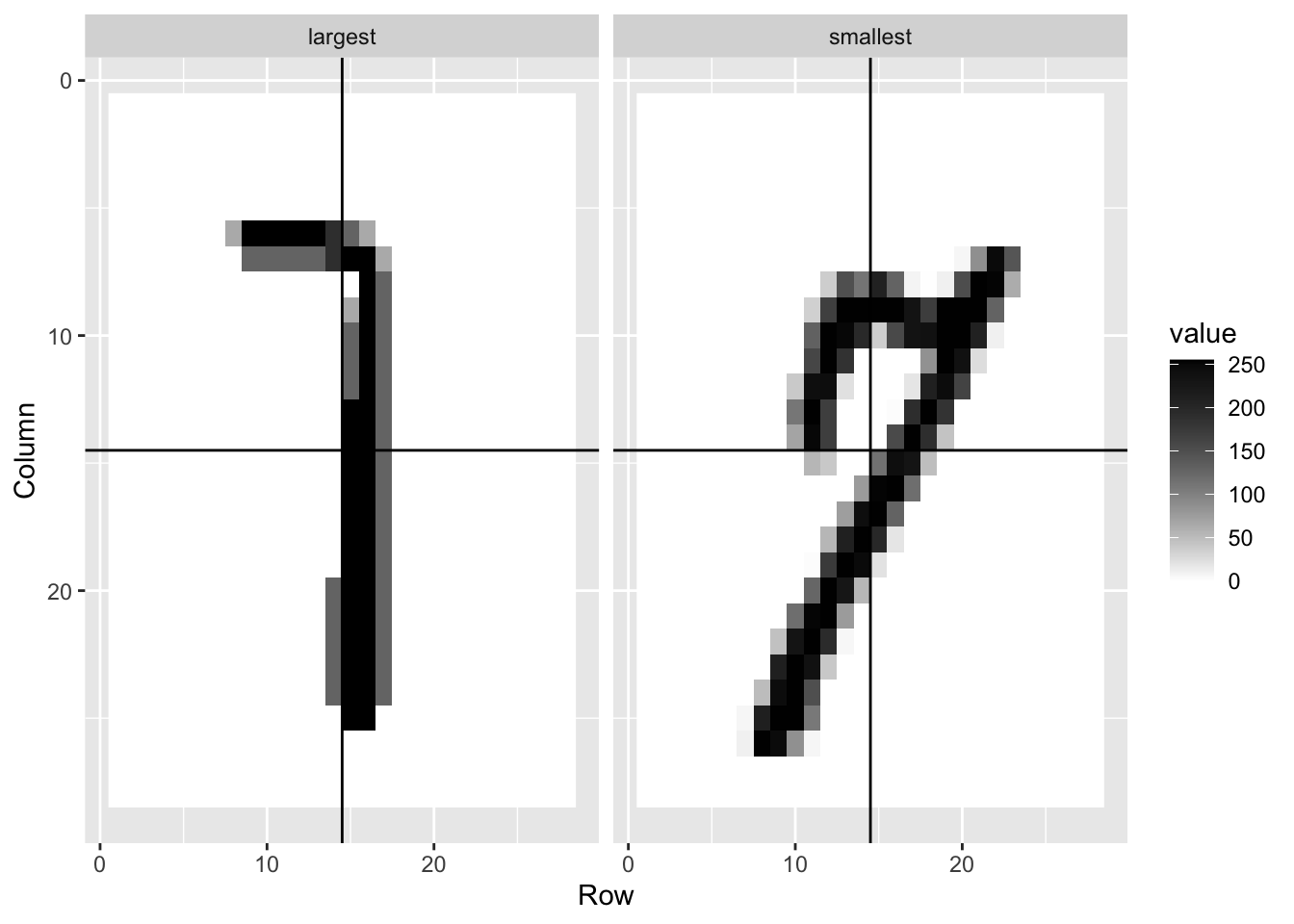

fit_glm <- glm(y ~ x_1 + x_2, data=mnist_27$train, family = "binomial")
p_hat_glm <- predict(fit_glm, mnist_27$test)
y_hat_glm <- factor(ifelse(p_hat_glm > 0.5, 7, 2))
confusionMatrix(data = y_hat_glm, reference = mnist_27$test$y)$overall["Accuracy"]

## Accuracy 
##     0.76

mnist_27$true_p %>% ggplot(aes(x_1, x_2, fill=p)) +
    geom_raster()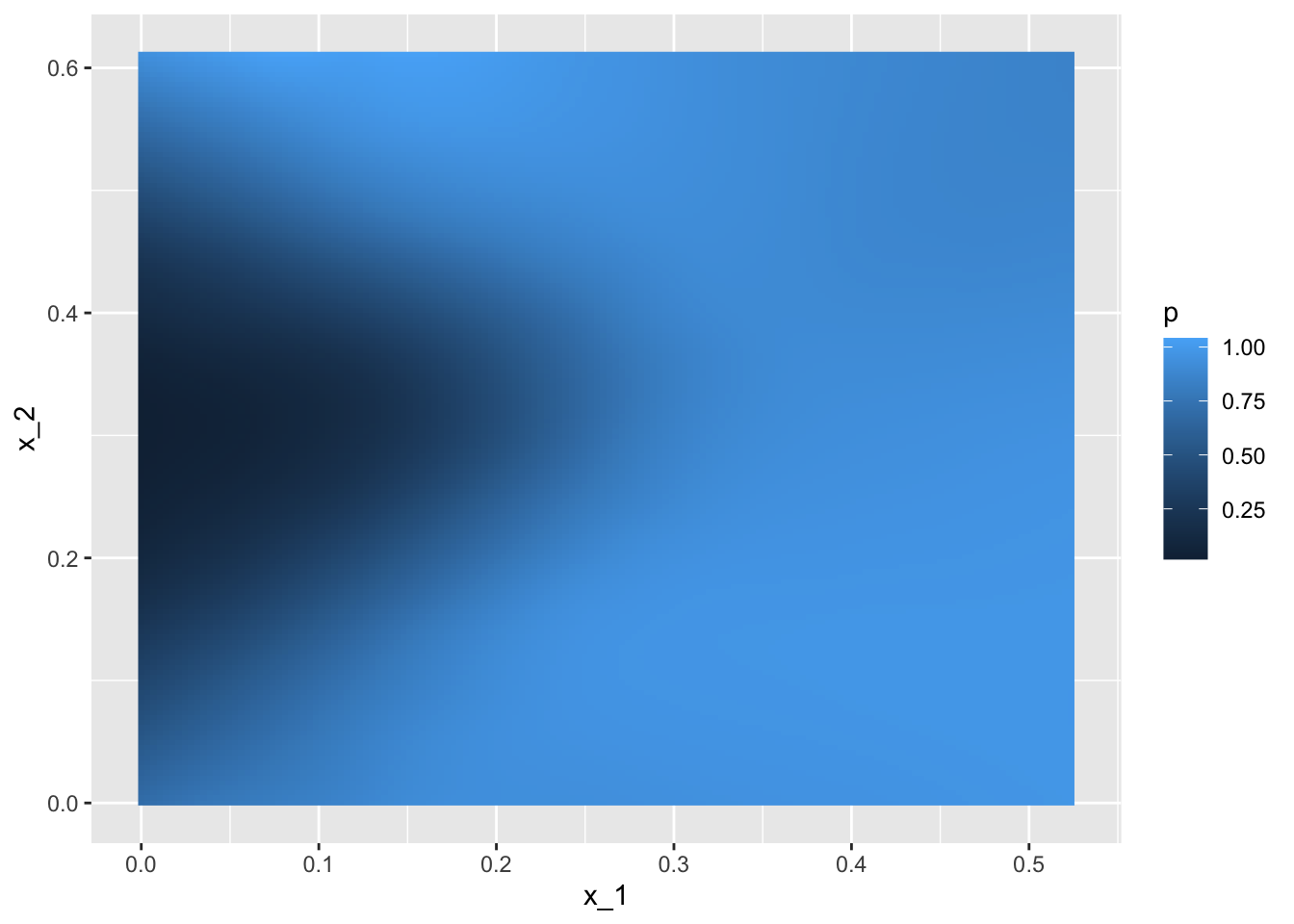

mnist_27$true_p %>% ggplot(aes(x_1, x_2, z=p, fill=p)) +
    geom_raster() +
    scale_fill_gradientn(colors=c("#F8766D","white","#00BFC4")) +
    stat_contour(breaks=c(0.5), color="black")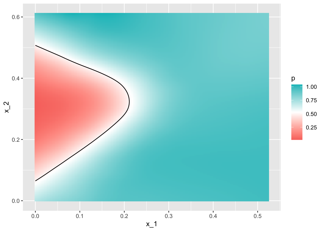 

p_hat <- predict(fit_glm, newdata = mnist_27$true_p)
mnist_27$true_p %>%
    mutate(p_hat = p_hat) %>%
    ggplot(aes(x_1, x_2,  z=p_hat, fill=p_hat)) +
    geom_raster() +
    scale_fill_gradientn(colors=c("#F8766D","white","#00BFC4")) +
    stat_contour(breaks=c(0.5),color="black")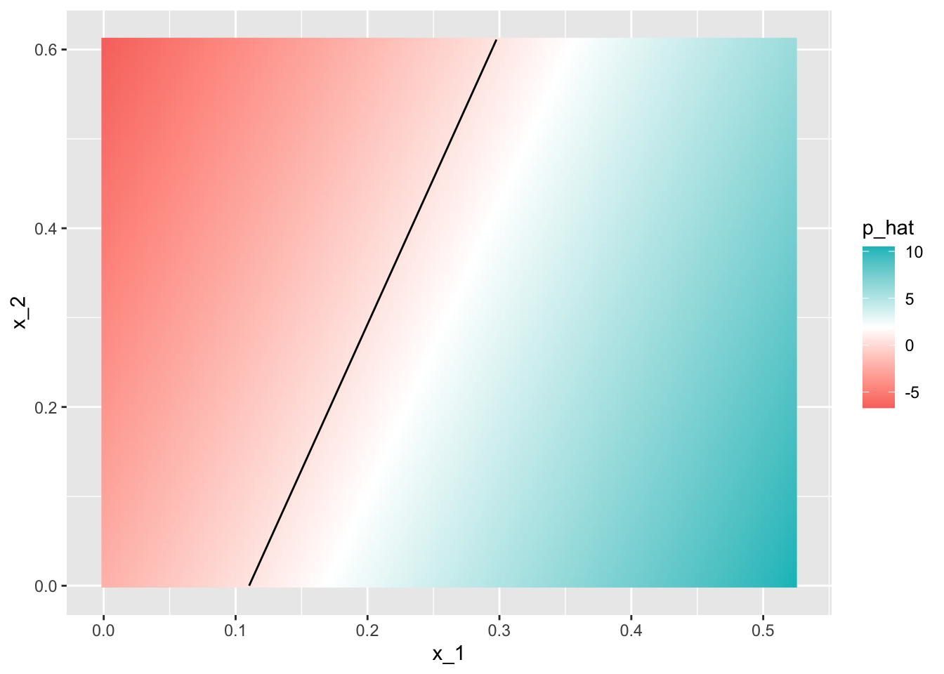 

p_hat <- predict(fit_glm, newdata = mnist_27$true_p)
mnist_27$true_p %>%
    mutate(p_hat = p_hat) %>%
    ggplot() +
    stat_contour(aes(x_1, x_2, z=p_hat), breaks=c(0.5), color="black") +
    geom_point(mapping = aes(x_1, x_2, color=y), data = mnist_27$test)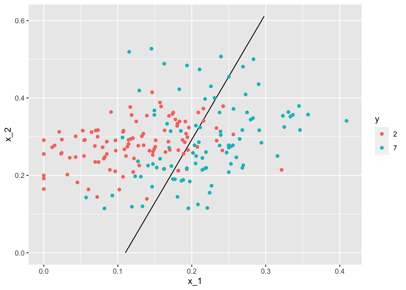

4.7 Comprehension Check - Logistic Regression

1. Define a dataset using the following code:

# set.seed(2) #if you are using R 3.5 or earlier
set.seed(2, sample.kind="Rounding") #if you are using R 3.6 or later

## Warning in set.seed(2, sample.kind = "Rounding"): non-uniform 'Rounding' sampler used

make_data <- function(n = 1000, p = 0.5, 
                mu_0 = 0, mu_1 = 2, 
                sigma_0 = 1,  sigma_1 = 1){

y <- rbinom(n, 1, p)
f_0 <- rnorm(n, mu_0, sigma_0)
f_1 <- rnorm(n, mu_1, sigma_1)
x <- ifelse(y == 1, f_1, f_0)
  
test_index <- createDataPartition(y, times = 1, p = 0.5, list = FALSE)

list(train = data.frame(x = x, y = as.factor(y)) %>% slice(-test_index),
    test = data.frame(x = x, y = as.factor(y)) %>% slice(test_index))
}
dat <- make_data()

Note that we have defined a variable x that is predictive of a binary outcome y:

dat$train %>% ggplot(aes(x, color = y)) + geom_density().

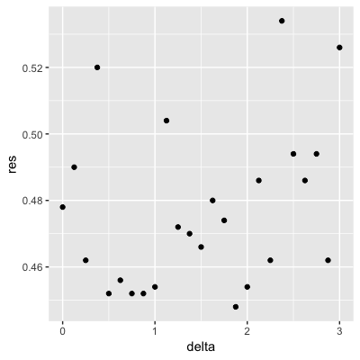
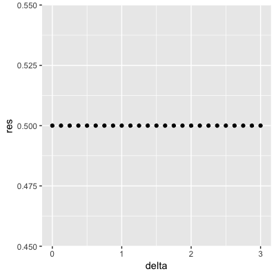
Set the seed to 1, then use the make_data() function defined above to generate 25 different datasets with mu_1 <- seq(0, 3, len=25). Perform logistic regression on each of the 25 different datasets (predict 1 if p > 0.5) and plot accuracy (res in the figures) vs mu_1 (delta in the figures).

Which is the correct plot?

set.seed(1) #if you are using R 3.5 or earlier
set.seed(1, sample.kind="Rounding") #if you are using R 3.6 or later

## Warning in set.seed(1, sample.kind = "Rounding"): non-uniform 'Rounding' sampler used

delta <- seq(0, 3, len = 25)
res <- sapply(delta, function(d){
    dat <- make_data(mu_1 = d)
    fit_glm <- dat$train %>% glm(y ~ x, family = "binomial", data = .)
    y_hat_glm <- ifelse(predict(fit_glm, dat$test) > 0.5, 1, 0) %>% factor(levels = c(0, 1))
    mean(y_hat_glm == dat$test$y)
})
qplot(delta, res)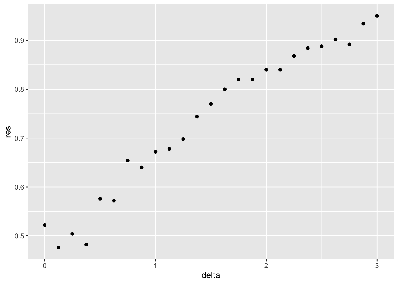

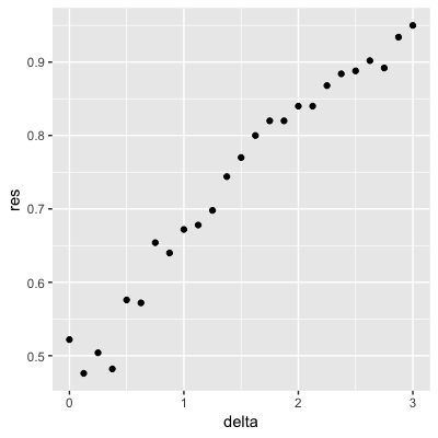
• A.

• B.

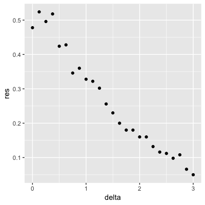
• C.

• D.

4.8 Introduction to Smoothing

There is a link to the relevant section of the textbook: Smoothing

Key points

• Smoothing is a very powerful technique used all across data analysis. It is designed to detect trends in the presence of noisy data in cases in which the shape of the trend is unknown.
• The concepts behind smoothing techniques are extremely useful in machine learning because conditional expectations/probabilities can be thought of as trends of unknown shapes that we need to estimate in the presence of uncertainty.

Code

data("polls_2008")
qplot(day, margin, data = polls_2008)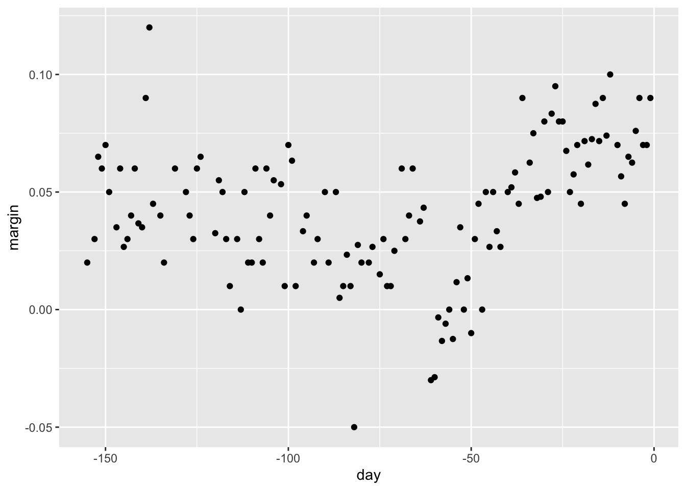

4.9 Bin Smoothing and Kernels

There is a link to the relevant sections of the textbook: Bin smoothing and Kernels

Key points

• The general idea of smoothing is to group data points into strata in which the value of \(f(x)\) can be assumed to be constant. We can make this assumption because we think \(f(x)\) changes slowly and, as a result, \(f(x)\) is almost constant in small windows of time.
• This assumption implies that a good estimate for \(f(x)\) is the average of the \(Y_{i}\) values in the window. The estimate is:

\(\hat{f}(x_{0})=\frac{1}{N_{0}}\sum_{i\in{A_{0}}}Y_{i}\)

• In smoothing, we call the size of the interval \(|x-x_{0}|\) satisfying the particular condition the window size, bandwidth or span.

Code

# bin smoothers
span <- 7 
fit <- with(polls_2008,ksmooth(day, margin, x.points = day, kernel="box", bandwidth =span))
polls_2008 %>% mutate(smooth = fit$y) %>%
    ggplot(aes(day, margin)) +
    geom_point(size = 3, alpha = .5, color = "grey") + 
    geom_line(aes(day, smooth), color="red")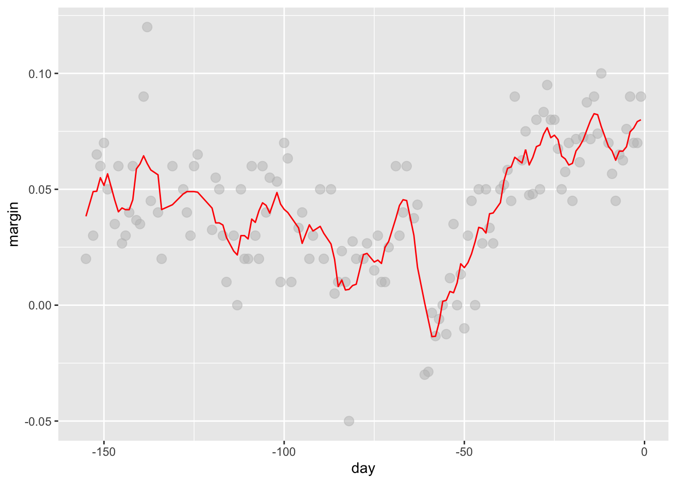

# kernel
span <- 7
fit <- with(polls_2008, ksmooth(day, margin,  x.points = day, kernel="normal", bandwidth = span))
polls_2008 %>% mutate(smooth = fit$y) %>%
  ggplot(aes(day, margin)) +
  geom_point(size = 3, alpha = .5, color = "grey") + 
  geom_line(aes(day, smooth), color="red")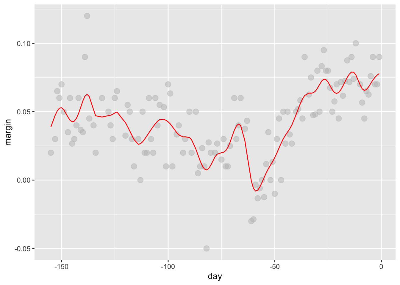

4.10 Local Weighted Regression (loess)

There is a link to the relevant section of the textbook: Local weighted regression

Key points

• A limitation of the bin smoothing approach is that we need small windows for the approximately constant assumptions to hold which may lead to imprecise estimates of \(f(x)\). Local weighted regression (loess) permits us to consider larger window sizes.
• One important difference between loess and bin smoother is that we assume the smooth function is locally linear in a window instead of constant.
• The result of loess is a smoother fit than bin smoothing because we use larger sample sizes to estimate our local parameters.

Code

polls_2008 %>% ggplot(aes(day, margin)) +
  geom_point() + 
  geom_smooth(color="red", span = 0.15, method = "loess", method.args = list(degree=1))

## `geom_smooth()` using formula 'y ~ x'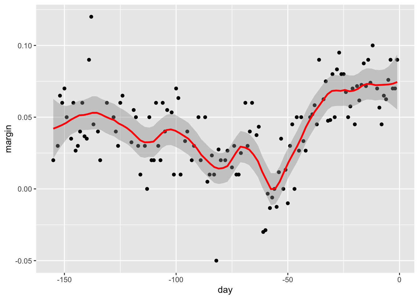

4.11 Comprehension Check - Smoothing

1. In the Wrangling course of this series, PH125.6x, we used the following code to obtain mortality counts for Puerto Rico for 2015-2018:

if(!require(purrr)) install.packages("purrr")
if(!require(pdftools)) install.packages("pdftools")

## Loading required package: pdftools

## Using poppler version 0.73.0

library(tidyverse)
library(lubridate)
library(purrr)
library(pdftools)
    
fn <- system.file("extdata", "RD-Mortality-Report_2015-18-180531.pdf", package="dslabs")
dat <- map_df(str_split(pdf_text(fn), "\n"), function(s){
    s <- str_trim(s)
    header_index <- str_which(s, "2015")[1]
    tmp <- str_split(s[header_index], "\\s+", simplify = TRUE)
    month <- tmp[1]
    header <- tmp[-1]
    tail_index  <- str_which(s, "Total")
    n <- str_count(s, "\\d+")
    out <- c(1:header_index, which(n==1), which(n>=28), tail_index:length(s))
    s[-out] %>%
        str_remove_all("[^\\d\\s]") %>%
        str_trim() %>%
        str_split_fixed("\\s+", n = 6) %>%
        .[,1:5] %>%
        as_data_frame() %>% 
        setNames(c("day", header)) %>%
        mutate(month = month,
            day = as.numeric(day)) %>%
        gather(year, deaths, -c(day, month)) %>%
        mutate(deaths = as.numeric(deaths))
}) %>%
    mutate(month = recode(month, "JAN" = 1, "FEB" = 2, "MAR" = 3, "APR" = 4, "MAY" = 5, "JUN" = 6, 
                          "JUL" = 7, "AGO" = 8, "SEP" = 9, "OCT" = 10, "NOV" = 11, "DEC" = 12)) %>%
    mutate(date = make_date(year, month, day)) %>%
        dplyr::filter(date <= "2018-05-01")

## Warning: `as_data_frame()` is deprecated as of tibble 2.0.0.
## Please use `as_tibble()` instead.
## The signature and semantics have changed, see `?as_tibble`.
## This warning is displayed once every 8 hours.
## Call `lifecycle::last_warnings()` to see where this warning was generated.

## Warning: The `x` argument of `as_tibble.matrix()` must have unique column names if `.name_repair` is omitted as of tibble 2.0.0.
## Using compatibility `.name_repair`.
## This warning is displayed once every 8 hours.
## Call `lifecycle::last_warnings()` to see where this warning was generated.

Use the loess() function to obtain a smooth estimate of the expected number of deaths as a function of date. Plot this resulting smooth function. Make the span about two months long.

Which of the following plots is correct?

span <- 60 / as.numeric(diff(range(dat$date)))
fit <- dat %>% mutate(x = as.numeric(date)) %>% loess(deaths ~ x, data = ., span = span, degree = 1)
dat %>% mutate(smooth = predict(fit, as.numeric(date))) %>%
    ggplot() +
    geom_point(aes(date, deaths)) +
    geom_line(aes(date, smooth), lwd = 2, col = "red")

## Warning: Removed 1 rows containing missing values (geom_point).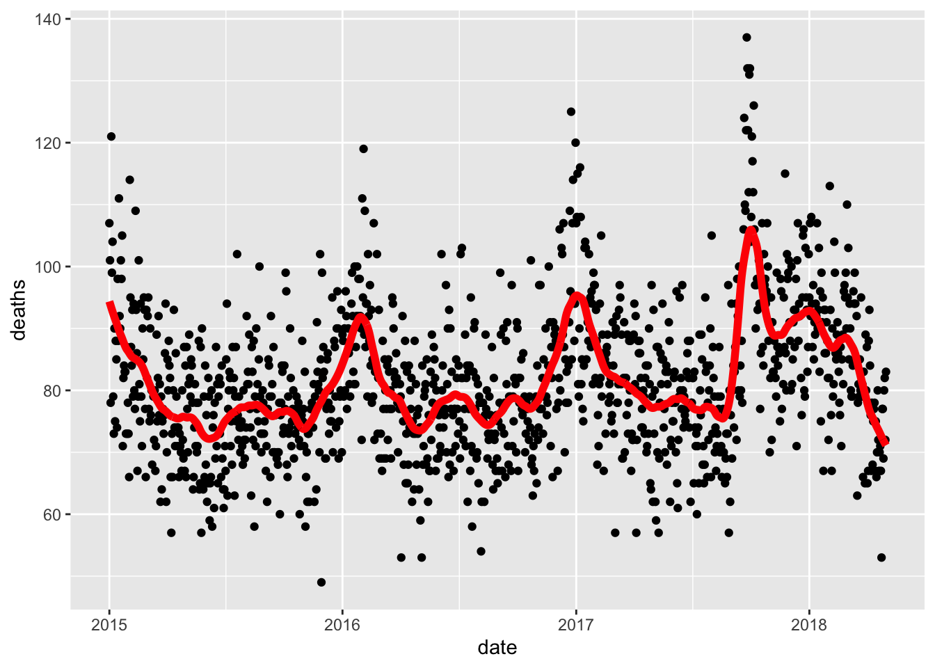

• A.

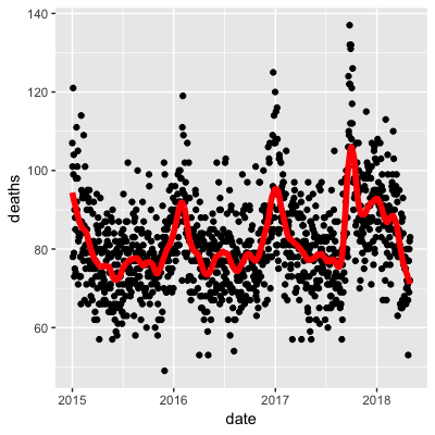
• B.

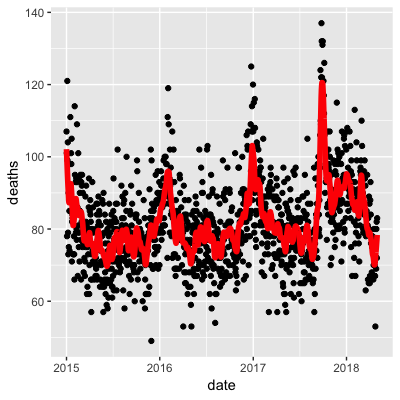
• C.

• D.

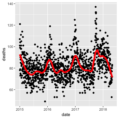
2. Work with the same data as in Q1 to plot smooth estimates against day of the year, all on the same plot, but with different colors for each year.

Which code produces the desired plot?

dat %>% 
    mutate(smooth = predict(fit, as.numeric(date)), day = yday(date), year = as.character(year(date))) %>%
    ggplot(aes(day, smooth, col = year)) +
    geom_line(lwd = 2)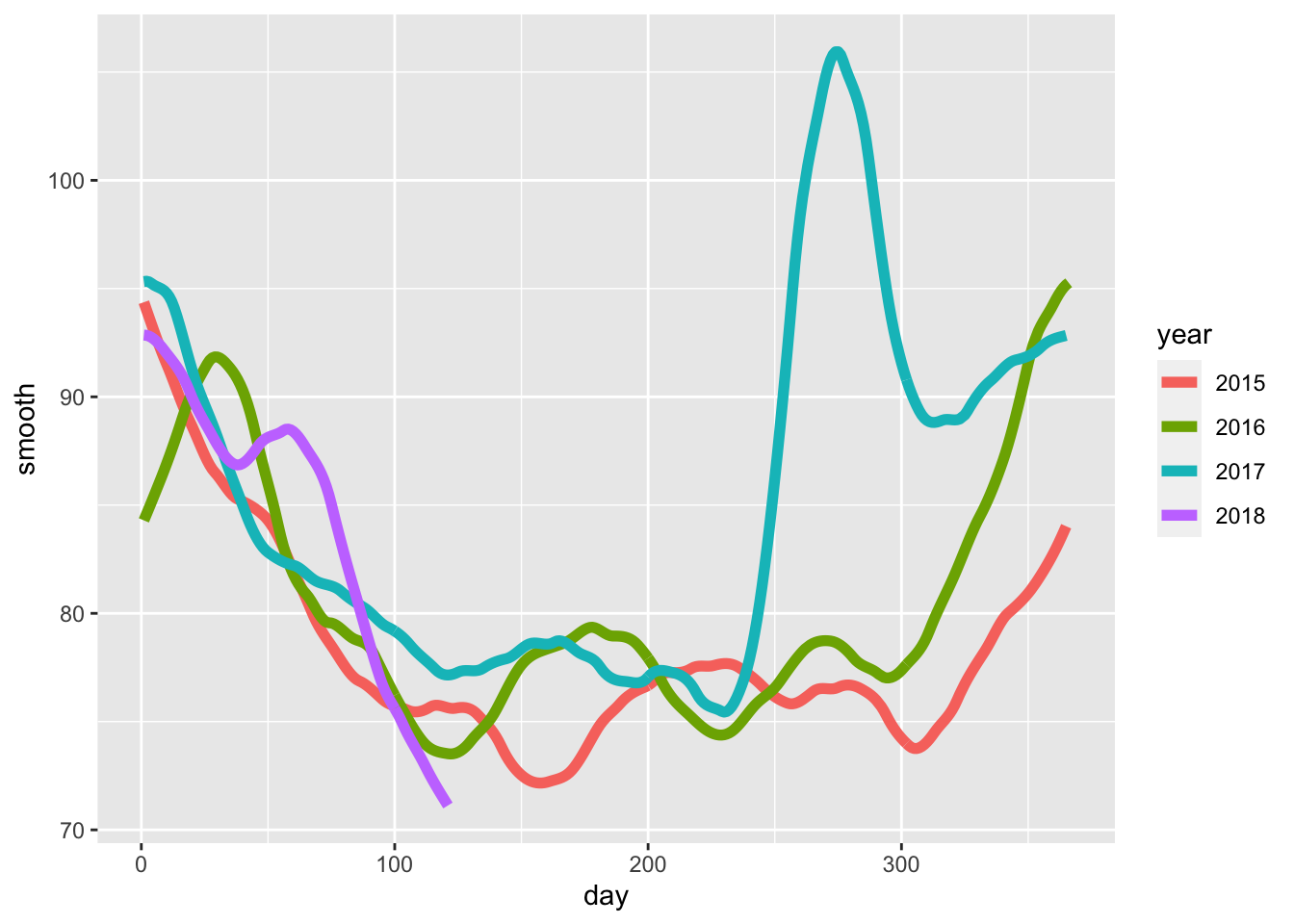

• A.

dat %>% 
    mutate(smooth = predict(fit), day = yday(date), year = as.character(year(date))) %>%
    ggplot(aes(day, smooth, col = year)) +
    geom_line(lwd = 2)

• B.

dat %>% 
    mutate(smooth = predict(fit, as.numeric(date)), day = mday(date), year = as.character(year(date))) %>%
    ggplot(aes(day, smooth, col = year)) +
    geom_line(lwd = 2)

• C.

 dat %>% 
    mutate(smooth = predict(fit, as.numeric(date)), day = yday(date), year = as.character(year(date))) %>%
    ggplot(aes(day, smooth)) +
    geom_line(lwd = 2)

• D.

dat %>% 
    mutate(smooth = predict(fit, as.numeric(date)), day = yday(date), year = as.character(year(date))) %>%
    ggplot(aes(day, smooth, col = year)) +
    geom_line(lwd = 2)

3. Suppose we want to predict 2s and 7s in the mnist_27 dataset with just the second covariate. Can we do this? On first inspection it appears the data does not have much predictive power.

In fact, if we fit a regular logistic regression the coefficient for x_2 is not significant!

This can be seen using this code:

if(!require(broom)) install.packages("broom")

## Loading required package: broom

library(broom)
mnist_27$train %>% glm(y ~ x_2, family = "binomial", data = .) %>% tidy()

## # A tibble: 2 x 5
##   term        estimate std.error statistic p.value
##   <chr>          <dbl>     <dbl>     <dbl>   <dbl>
## 1 (Intercept)  -0.0907     0.247    -0.368   0.713
## 2 x_2           0.685      0.827     0.829   0.407

Plotting a scatterplot here is not useful since y is binary:

qplot(x_2, y, data = mnist_27$train)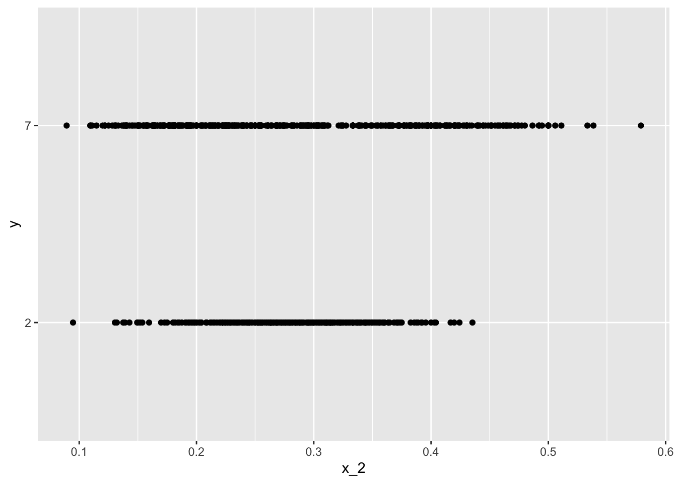

Fit a loess line to the data above and plot the results. What do you observe?

mnist_27$train %>% 
    mutate(y = ifelse(y=="7", 1, 0)) %>%
    ggplot(aes(x_2, y)) + 
    geom_smooth(method = "loess")

## `geom_smooth()` using formula 'y ~ x'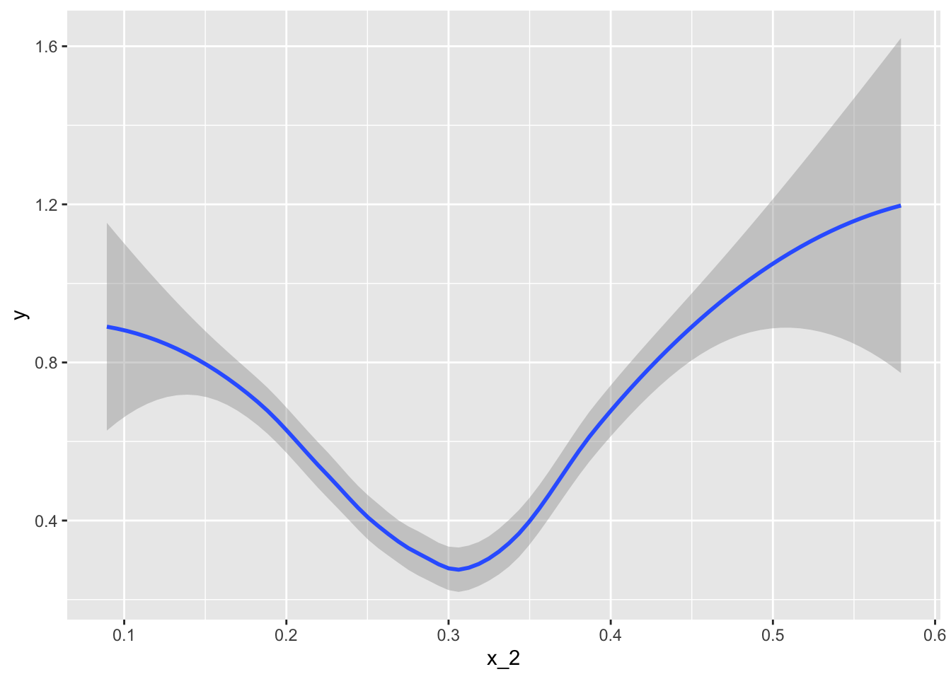

• A. There is no predictive power and the conditional probability is linear.
• B. There is no predictive power and the conditional probability is non-linear.
• C. There is predictive power and the conditional probability is linear.
• D. There is predictive power and the conditional probability is non-linear.

4.12 Matrices

There is a link to the relevant section of the textbook: Matrices

Key points

• The main reason for using matrices is that certain mathematical operations needed to develop efficient code can be performed using techniques from a branch of mathematics called linear algebra.
• Linear algebra and matrix notation are key elements of the language used in academic papers describing machine learning techniques.

Code

if(!exists("mnist")) mnist <- read_mnist()

class(mnist$train$images)

## [1] "matrix" "array"

x <- mnist$train$images[1:1000,] 
y <- mnist$train$labels[1:1000]

4.13 Matrix Notation

There is a link to the relevant section of the textbook: Matrix notation

Key points

• In matrix algebra, we have three main types of objects: scalars, vectors, and matrices.
  • Scalar: \(\alpha=1\)
  • Vector: \(X_{1} = \left(\begin{matrix} x_{1,1} \\ \vdots \\ x_{N,1} \\ \end{matrix}\right)\)
  • Matrix: \(X = [X_{1}X_{2}] = \left(\begin{matrix} x_{1,1} & x_{1,2} \\ \vdots & \vdots \\ x_{N,1} & x_{N,2} \\ \end{matrix}\right)\)
• In R, we can extract the dimension of a matrix with the function dim(). We can convert a vector into a matrix using the function as.matrix().

Code

length(x[,1])

## [1] 1000

x_1 <- 1:5
x_2 <- 6:10
cbind(x_1, x_2)

##      x_1 x_2
## [1,]   1   6
## [2,]   2   7
## [3,]   3   8
## [4,]   4   9
## [5,]   5  10

dim(x)

## [1] 1000  784

dim(x_1)

## NULL

dim(as.matrix(x_1))

## [1] 5 1

dim(x)

## [1] 1000  784

4.14 Converting a Vector to a Matrix

There is a link to the relevant section of the textbook: Converting a vector to a matrix

Key points

• In R, we can convert a vector into a matrix with the matrix() function. The matrix is filled in by column, but we can fill by row by using the byrow argument. The function t() can be used to directly transpose a matrix.
• Note that the matrix function recycles values in the vector without warning if the product of columns and rows does not match the length of the vector.

Code

my_vector <- 1:15

# fill the matrix by column
mat <- matrix(my_vector, 5, 3)
mat

##      [,1] [,2] [,3]
## [1,]    1    6   11
## [2,]    2    7   12
## [3,]    3    8   13
## [4,]    4    9   14
## [5,]    5   10   15

# fill by row
mat_t <- matrix(my_vector, 3, 5, byrow = TRUE)
mat_t

##      [,1] [,2] [,3] [,4] [,5]
## [1,]    1    2    3    4    5
## [2,]    6    7    8    9   10
## [3,]   11   12   13   14   15

identical(t(mat), mat_t)

## [1] TRUE

matrix(my_vector, 5, 5)

##      [,1] [,2] [,3] [,4] [,5]
## [1,]    1    6   11    1    6
## [2,]    2    7   12    2    7
## [3,]    3    8   13    3    8
## [4,]    4    9   14    4    9
## [5,]    5   10   15    5   10

grid <- matrix(x[3,], 28, 28)
image(1:28, 1:28, grid)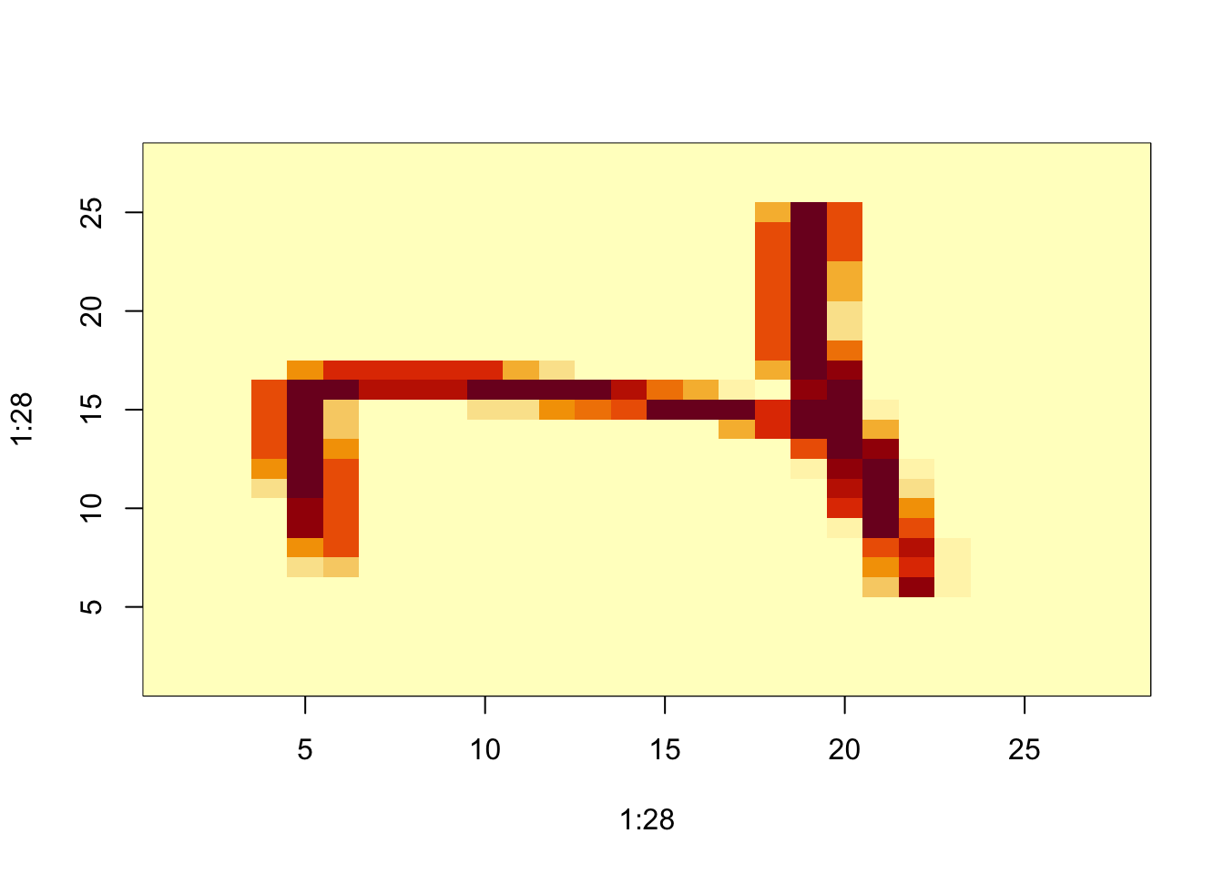

# flip the image back
image(1:28, 1:28, grid[, 28:1])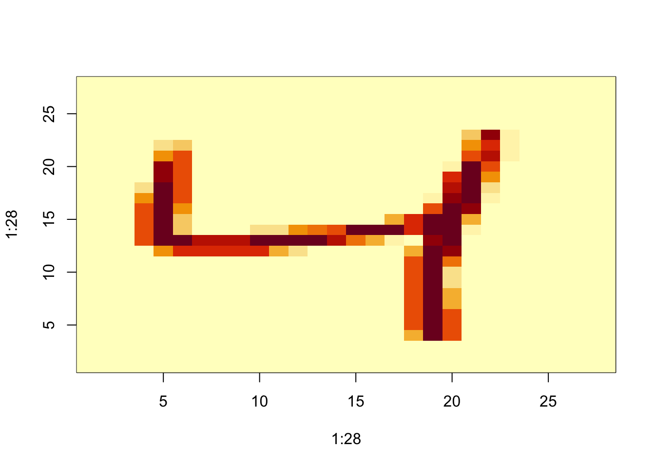

4.15 Row and Column Summaries and Apply

There is a link to the relevant section of the textbook: Row and column summaries

Key points

• The function rowSums() computes the sum of each row.
• The function rowMeans() computes the average of each row.
• We can compute the column sums and averages using the functions colSums() and colMeans().
• The matrixStats package adds functions that performs operations on each row or column very efficiently, including the functions rowSds() and colSds().
• The apply() function lets you apply any function to a matrix. The first argument is the matrix, the second is the dimension (1 for rows, 2 for columns), and the third is the function.

Code

sums <- rowSums(x)
avg <- rowMeans(x)

data_frame(labels = as.factor(y), row_averages = avg) %>%
    qplot(labels, row_averages, data = ., geom = "boxplot")

## Warning: `data_frame()` is deprecated as of tibble 1.1.0.
## Please use `tibble()` instead.
## This warning is displayed once every 8 hours.
## Call `lifecycle::last_warnings()` to see where this warning was generated.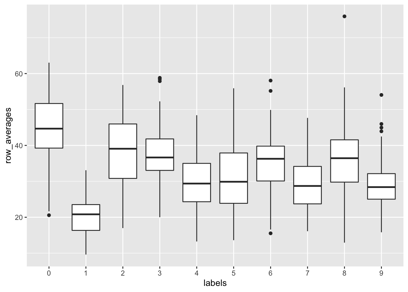

avgs <- apply(x, 1, mean)
sds <- apply(x, 2, sd)

4.16 Filtering Columns Based on Summaries

There is a link to the relevant section of the textbook: Filtering columns based on summaries

Key points

• The operations used to extract columns: x[,c(351,352)].
• The operations used to extract rows: x[c(2,3),].
• We can also use logical indexes to determine which columns or rows to keep: new_x <- x[ ,colSds(x) > 60].
• Important note: if you select only one column or only one row, the result is no longer a matrix but a vector. We can preserve the matrix class by using the argument drop=FALSE.

Code

if(!require(matrixStats)) install.packages("matrixStats")

## Loading required package: matrixStats

## 
## Attaching package: 'matrixStats'

## The following object is masked from 'package:dplyr':
## 
##     count

library(matrixStats)

sds <- colSds(x)
qplot(sds, bins = "30", color = I("black"))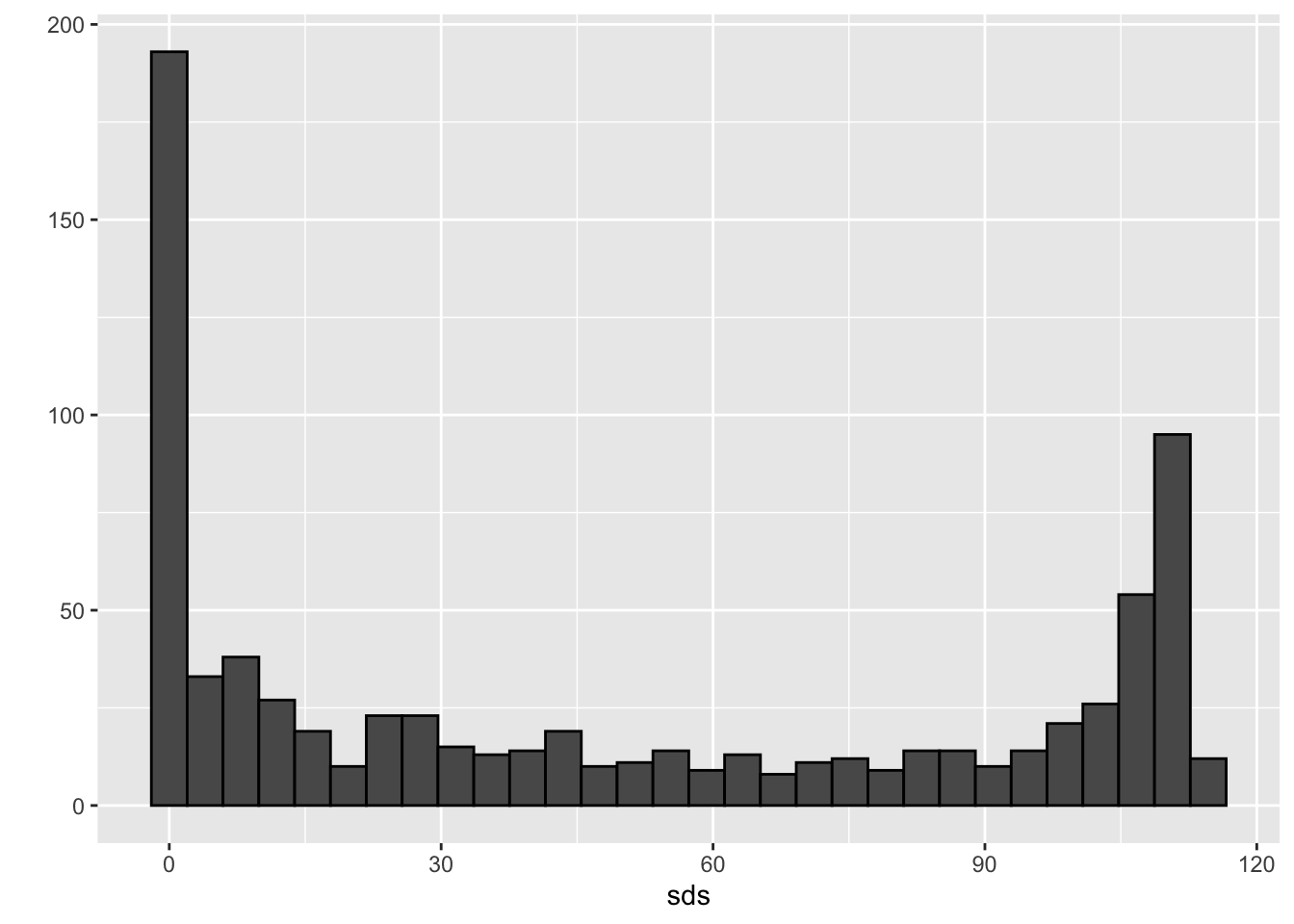

image(1:28, 1:28, matrix(sds, 28, 28)[, 28:1])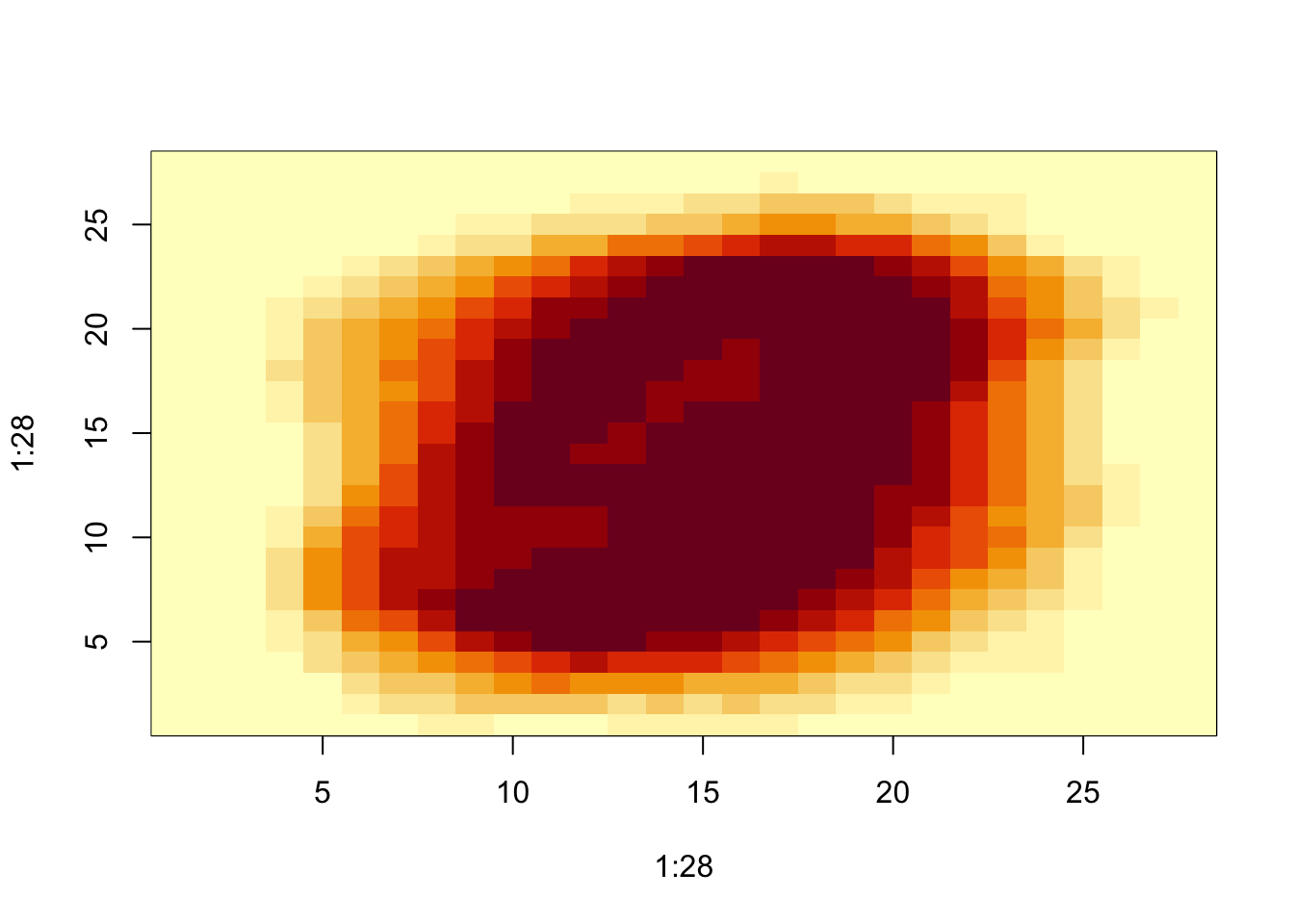

#extract columns and rows
x[ ,c(351,352)]

##         [,1] [,2]
##    [1,]   70    0
##    [2,]    0    0
##    [3,]    0    0
##    [4,]  205  253
##    [5,]    8   78
##    [6,]    0    0
##    [7,]  253  253
##    [8,]   91  212
##    [9,]  254  143
##   [10,]    0    0
##   [11,]  254  254
##   [12,]   78   79
##   [13,]  254  248
##   [14,]    0  114
##   [15,]  254  109
##   [16,]    0    0
##   [17,]    0    0
##   [18,]   80  223
##   [19,]    0    0
##   [20,]    8   43
##   [21,]  109  109
##   [22,]   96  204
##   [23,]    0    0
##   [24,]  142  255
##   [25,]   32  254
##   [26,]  250  253
##   [27,]    0    0
##   [28,]  253  253
##   [29,]    0    0
##   [30,]    2    0
##   [31,]  253  253
##   [32,]  253  253
##   [33,]    0    0
##   [34,]  228  216
##   [35,]  225    0
##   [36,]  141   86
##   [37,]  107    0
##   [38,]    0    0
##   [39,]    0   15
##   [40,]    0    0
##   [41,]  253  253
##   [42,]  232  233
##   [43,]    0  182
##   [44,]   71  173
##   [45,]  253  203
##   [46,]   44  199
##   [47,]    0  154
##   [48,]    0    0
##   [49,]  169  254
##   [50,]  252  176
##   [51,]  254  254
##   [52,]    0    0
##   [53,]    0    0
##   [54,]   24  242
##   [55,]   71  122
##   [56,]    0  186
##   [57,]    0    0
##   [58,]    0    0
##   [59,]  111  189
##   [60,]  229  254
##   [61,]    0    0
##   [62,]    0  227
##   [63,]    0    0
##   [64,]  253  251
##   [65,]    0    0
##   [66,]  216  151
##   [67,]  128  128
##   [68,]  254  254
##   [69,]    0    0
##   [70,]   29    0
##   [71,]  253  122
##   [72,]   69    0
##   [73,]  254  204
##   [74,]   17  179
##   [75,]  253  252
##   [76,]  182   15
##   [77,]  254  254
##   [78,]  251  253
##   [79,]  173  253
##   [80,]   10    0
##   [81,]  252  253
##   [82,]    0    0
##   [83,]    0    0
##   [84,]    0  128
##   [85,]    0    0
##   [86,]  253  253
##   [87,]  253  253
##   [88,]   21   52
##   [89,]    0    0
##   [90,]    0    0
##   [91,]    0    0
##   [92,]   53   53
##   [93,]    0    0
##   [94,]   70  236
##   [95,]   38    0
##   [96,]    0    0
##   [97,]    0   26
##   [98,]   38   38
##   [99,]  253  240
##  [100,]   69  253
##  [101,]    0    0
##  [102,]   66    0
##  [103,]  254   95
##  [104,]    0    0
##  [105,]  251    0
##  [106,]  253  253
##  [107,]    0    0
##  [108,]  191  255
##  [109,]    0    0
##  [110,]  163    8
##  [111,]   78  253
##  [112,]   55  139
##  [113,]  252  253
##  [114,]  252  252
##  [115,]    0    0
##  [116,]    0    0
##  [117,]    0   15
##  [118,]  253  253
##  [119,]    0    0
##  [120,]   14    0
##  [121,]    0    0
##  [122,]    0    0
##  [123,]    0  150
##  [124,]    0    0
##  [125,]  253  233
##  [126,]  254  178
##  [127,]    0    0
##  [128,]   61    1
##  [129,]  253  253
##  [130,]  192  252
##  [131,]  254  247
##  [132,]    0    5
##  [133,]  253  253
##  [134,]  141  240
##  [135,]  253  251
##  [136,]  252  252
##  [137,]  254  179
##  [138,]  255  255
##  [139,]  244  253
##  [140,]    0    0
##  [141,]    0    0
##  [142,]  131   44
##  [143,]    0    0
##  [144,]  162  255
##  [145,]   72  142
##  [146,]    0    0
##  [147,]    0   34
##  [148,]    0    0
##  [149,]    0    0
##  [150,]  252  252
##  [151,]  221  254
##  [152,]    0    0
##  [153,]  232  254
##  [154,]    5   89
##  [155,]  253  213
##  [156,]    0   36
##  [157,]    0    0
##  [158,]  179  242
##  [159,]   50   50
##  [160,]    0   90
##  [161,]  254  254
##  [162,]  229  254
##  [163,]    0    0
##  [164,]   76  243
##  [165,]    0    0
##  [166,]   63  167
##  [167,]    0    0
##  [168,]    0    0
##  [169,]  253  252
##  [170,]  105    4
##  [171,]   37  168
##  [172,]   69  168
##  [173,]  255  152
##  [174,]  170    0
##  [175,]  252  253
##  [176,]  185    8
##  [177,]  254  253
##  [178,]  251  253
##  [179,]    0    0
##  [180,]   59  106
##  [181,]    0  178
##  [182,]    0    0
##  [183,]  176  253
##  [184,]    0   64
##  [185,]  253  226
##  [186,]    0    0
##  [187,]    0    0
##  [188,]  254  254
##  [189,]    0    0
##  [190,]  252  252
##  [191,]  167  254
##  [192,]    0    0
##  [193,]    0    0
##  [194,]   32   32
##  [195,]    0    0
##  [196,]  148  149
##  [197,]    0    0
##  [198,]  250  225
##  [199,]  104  252
##  [200,]    0   11
##  [201,]  253  169
##  [202,]  157  252
##  [203,]  100  247
##  [204,]  162  216
##  [205,]    0    0
##  [206,]  253  251
##  [207,]    0    0
##  [208,]    0    0
##  [209,]  253  253
##  [210,]    0    0
##  [211,]    0    0
##  [212,]  253  254
##  [213,]  199  253
##  [214,]    0   20
##  [215,]    0    0
##  [216,]  253  253
##  [217,]    0    0
##  [218,]    0    0
##  [219,]  106  239
##  [220,]  181   84
##  [221,]    0    0
##  [222,]    0   31
##  [223,]  152  244
##  [224,]    0    0
##  [225,]    0   61
##  [226,]  253  227
##  [227,]    0  136
##  [228,]    0    0
##  [229,]    0    0
##  [230,]    0    0
##  [231,]    0    0
##  [232,]  253  251
##  [233,]    0    0
##  [234,]    0    0
##  [235,]    0    2
##  [236,]  253  253
##  [237,]    0    0
##  [238,]    0    0
##  [239,]    0    0
##  [240,]   98   88
##  [241,]  253  252
##  [242,]    0    0
##  [243,]  254  254
##  [244,]    0    0
##  [245,]    0  169
##  [246,]  255  255
##  [247,]    0    0
##  [248,]    0    2
##  [249,]  254  252
##  [250,]    0    0
##  [251,]    0    1
##  [252,]  253  253
##  [253,]  253  252
##  [254,]    0    0
##  [255,]  254  254
##  [256,]  253  253
##  [257,]  253  171
##  [258,]    0    0
##  [259,]    0    0
##  [260,]  254  231
##  [261,]    0    0
##  [262,]    0    0
##  [263,]    0    0
##  [264,]    0    0
##  [265,]    0    0
##  [266,]  236   62
##  [267,]   77    0
##  [268,]    0   90
##  [269,]    0   93
##  [270,]  253  253
##  [271,]  251   57
##  [272,]    0    0
##  [273,]  125  168
##  [274,]  127  127
##  [275,]  232    8
##  [276,]    0    0
##  [277,]  191  254
##  [278,]    0    0
##  [279,]  245  254
##  [280,]    0  128
##  [281,]    0   51
##  [282,]  253  255
##  [283,]    0    0
##  [284,]    0    0
##  [285,]  253  253
##  [286,]    0    0
##  [287,]  253  253
##  [288,]  254  251
##  [289,]    0    0
##  [290,]    0    0
##  [291,]  252  253
##  [292,]  253  253
##  [293,]    2   45
##  [294,]    0    0
##  [295,]    0    0
##  [296,]  133  160
##  [297,]    0    0
##  [298,]    0    0
##  [299,]  253  253
##  [300,]    0  155
##  [301,]   42  235
##  [302,]    0    0
##  [303,]    0    0
##  [304,]    0    0
##  [305,]   29   29
##  [306,]    0    0
##  [307,]  100  176
##  [308,]    0    0
##  [309,]    0    0
##  [310,]  232  253
##  [311,]  235  254
##  [312,]    0    0
##  [313,]  183  102
##  [314,]    0   35
##  [315,]    0    0
##  [316,]  243  253
##  [317,]  255  255
##  [318,]    0    0
##  [319,]  241  224
##  [320,]    0    5
##  [321,]    0    0
##  [322,]  230  253
##  [323,]    0    0
##  [324,]    0    0
##  [325,]    0    0
##  [326,]    0    0
##  [327,]    0    0
##  [328,]  253  253
##  [329,]   45    0
##  [330,]    0    0
##  [331,]   70   70
##  [332,]    0    0
##  [333,]    0    0
##  [334,]  184  184
##  [335,]    0  183
##  [336,]  211   86
##  [337,]    0    0
##  [338,]    0    0
##  [339,]    0    0
##  [340,]    0    0
##  [341,]    0   64
##  [342,]  253  255
##  [343,]  132  152
##  [344,]  252  241
##  [345,]    0    0
##  [346,]  158  254
##  [347,]    8  134
##  [348,]    0    0
##  [349,]  205  254
##  [350,]    0    0
##  [351,]    0    3
##  [352,]  180  253
##  [353,]  253  207
##  [354,]    0    0
##  [355,]    0  102
##  [356,]  254  254
##  [357,]  253  253
##  [358,]  211  253
##  [359,]  254   95
##  [360,]    0    0
##  [361,]  253  253
##  [362,]  160  252
##  [363,]    0    0
##  [364,]    0   96
##  [365,]    0    0
##  [366,]    0    0
##  [367,]  253  217
##  [368,]    0    0
##  [369,]  254  254
##  [370,]    0    0
##  [371,]  253  253
##  [372,]    0    0
##  [373,]    0   43
##  [374,]    0    0
##  [375,]  121  252
##  [376,]    0    0
##  [377,]    0    0
##  [378,]    0    0
##  [379,]    0    0
##  [380,]    0    3
##  [381,]    0    0
##  [382,]    0    0
##  [383,]  254   84
##  [384,]    0    0
##  [385,]    0   56
##  [386,]    0   52
##  [387,]  252  240
##  [388,]    0    0
##  [389,]    0    0
##  [390,]    0    0
##  [391,]   38  233
##  [392,]  197  173
##  [393,]   53  232
##  [394,]   64   64
##  [395,]  181    0
##  [396,]    0    0
##  [397,]    0    0
##  [398,]  207  252
##  [399,]  253  158
##  [400,]   27    0
##  [401,]    0    0
##  [402,]    0    0
##  [403,]    0    0
##  [404,]  105    0
##  [405,]  253  253
##  [406,]   93  239
##  [407,]  253   58
##  [408,]   42   27
##  [409,]  254  195
##  [410,]    0    0
##  [411,]  229  253
##  [412,]    0    0
##  [413,]    0  100
##  [414,]    0    0
##  [415,]    0   70
##  [416,]    0    0
##  [417,]  253  251
##  [418,]   58    0
##  [419,]    7  221
##  [420,]    0   45
##  [421,]  252  253
##  [422,]    0    0
##  [423,]    0   77
##  [424,]    0    0
##  [425,]  253  253
##  [426,]   23   29
##  [427,]  252  252
##  [428,]    0    0
##  [429,]  135  246
##  [430,]    0    0
##  [431,]    0    0
##  [432,]    0    0
##  [433,]    0    0
##  [434,]  253  253
##  [435,]    0    0
##  [436,]    0    0
##  [437,]    0    0
##  [438,]   40    8
##  [439,]    0   34
##  [440,]  254  254
##  [441,]    0    0
##  [442,]    0   47
##  [443,]    0    0
##  [444,]   99  253
##  [445,]  222  246
##  [446,]  252  209
##  [447,]    0    0
##  [448,]  172  253
##  [449,]   12  161
##  [450,]    0    0
##  [451,]  251  180
##  [452,]    0    0
##  [453,]  254  253
##  [454,]    0    0
##  [455,]  254  223
##  [456,]  237  252
##  [457,]  252  252
##  [458,]    0    0
##  [459,]    0    0
##  [460,]   49  159
##  [461,]    0    0
##  [462,]    0    0
##  [463,]    0    0
##  [464,]    0    0
##  [465,]    0    0
##  [466,]    0    0
##  [467,]   98  254
##  [468,]    0    0
##  [469,]    0    0
##  [470,]    0    0
##  [471,]    0    0
##  [472,]   51   51
##  [473,]  154  250
##  [474,]    0    0
##  [475,]    0    0
##  [476,]  211  253
##  [477,]    0    0
##  [478,]    0    0
##  [479,]  114  253
##  [480,]  254  253
##  [481,]    0    0
##  [482,]    0    0
##  [483,]    0    0
##  [484,]    0    0
##  [485,]  253  132
##  [486,]    0    0
##  [487,]   67    0
##  [488,]    0    9
##  [489,]  254  255
##  [490,]    0    0
##  [491,]  253  250
##  [492,]    0  255
##  [493,]  252  250
##  [494,]    0    0
##  [495,]    0    0
##  [496,]  253  253
##  [497,]  202  203
##  [498,]    0    0
##  [499,]    0    0
##  [500,]  130   76
##  [ reached getOption("max.print") -- omitted 500 rows ]

x[c(2,3),]

##      [,1] [,2] [,3] [,4] [,5] [,6] [,7] [,8] [,9] [,10] [,11] [,12] [,13] [,14] [,15] [,16] [,17] [,18] [,19] [,20] [,21] [,22] [,23] [,24] [,25] [,26] [,27] [,28] [,29] [,30] [,31]
## [1,]    0    0    0    0    0    0    0    0    0     0     0     0     0     0     0     0     0     0     0     0     0     0     0     0     0     0     0     0     0     0     0
##      [,32] [,33] [,34] [,35] [,36] [,37] [,38] [,39] [,40] [,41] [,42] [,43] [,44] [,45] [,46] [,47] [,48] [,49] [,50] [,51] [,52] [,53] [,54] [,55] [,56] [,57] [,58] [,59] [,60]
## [1,]     0     0     0     0     0     0     0     0     0     0     0     0     0     0     0     0     0     0     0     0     0     0     0     0     0     0     0     0     0
##      [,61] [,62] [,63] [,64] [,65] [,66] [,67] [,68] [,69] [,70] [,71] [,72] [,73] [,74] [,75] [,76] [,77] [,78] [,79] [,80] [,81] [,82] [,83] [,84] [,85] [,86] [,87] [,88] [,89]
## [1,]     0     0     0     0     0     0     0     0     0     0     0     0     0     0     0     0     0     0     0     0     0     0     0     0     0     0     0     0     0
##      [,90] [,91] [,92] [,93] [,94] [,95] [,96] [,97] [,98] [,99] [,100] [,101] [,102] [,103] [,104] [,105] [,106] [,107] [,108] [,109] [,110] [,111] [,112] [,113] [,114] [,115]
## [1,]     0     0     0     0     0     0     0     0     0     0      0      0      0      0      0      0      0      0      0      0      0      0      0      0      0      0
##      [,116] [,117] [,118] [,119] [,120] [,121] [,122] [,123] [,124] [,125] [,126] [,127] [,128] [,129] [,130] [,131] [,132] [,133] [,134] [,135] [,136] [,137] [,138] [,139] [,140]
## [1,]      0      0      0      0      0      0      0      0      0      0      0      0     51    159    253    159     50      0      0      0      0      0      0      0      0
##      [,141] [,142] [,143] [,144] [,145] [,146] [,147] [,148] [,149] [,150] [,151] [,152] [,153] [,154] [,155] [,156] [,157] [,158] [,159] [,160] [,161] [,162] [,163] [,164] [,165]
## [1,]      0      0      0      0      0      0      0      0      0      0      0      0      0      0     48    238    252    252    252    237      0      0      0      0      0
##      [,166] [,167] [,168] [,169] [,170] [,171] [,172] [,173] [,174] [,175] [,176] [,177] [,178] [,179] [,180] [,181] [,182] [,183] [,184] [,185] [,186] [,187] [,188] [,189] [,190]
## [1,]      0      0      0      0      0      0      0      0      0      0      0      0      0      0      0      0     54    227    253    252    239    233    252     57      6
##      [,191] [,192] [,193] [,194] [,195] [,196] [,197] [,198] [,199] [,200] [,201] [,202] [,203] [,204] [,205] [,206] [,207] [,208] [,209] [,210] [,211] [,212] [,213] [,214] [,215]
## [1,]      0      0      0      0      0      0      0      0      0      0      0      0      0      0      0      0      0     10     60    224    252    253    252    202     84
##      [,216] [,217] [,218] [,219] [,220] [,221] [,222] [,223] [,224] [,225] [,226] [,227] [,228] [,229] [,230] [,231] [,232] [,233] [,234] [,235] [,236] [,237] [,238] [,239] [,240]
## [1,]    252    253    122      0      0      0      0      0      0      0      0      0      0      0      0      0      0      0      0      0    163    252    252    252    253
##      [,241] [,242] [,243] [,244] [,245] [,246] [,247] [,248] [,249] [,250] [,251] [,252] [,253] [,254] [,255] [,256] [,257] [,258] [,259] [,260] [,261] [,262] [,263] [,264] [,265]
## [1,]    252    252     96    189    253    167      0      0      0      0      0      0      0      0      0      0      0      0      0      0      0      0     51    238    253
##      [,266] [,267] [,268] [,269] [,270] [,271] [,272] [,273] [,274] [,275] [,276] [,277] [,278] [,279] [,280] [,281] [,282] [,283] [,284] [,285] [,286] [,287] [,288] [,289] [,290]
## [1,]    253    190    114    253    228     47     79    255    168      0      0      0      0      0      0      0      0      0      0      0      0      0      0      0     48
##      [,291] [,292] [,293] [,294] [,295] [,296] [,297] [,298] [,299] [,300] [,301] [,302] [,303] [,304] [,305] [,306] [,307] [,308] [,309] [,310] [,311] [,312] [,313] [,314] [,315]
## [1,]    238    252    252    179     12     75    121     21      0      0    253    243     50      0      0      0      0      0      0      0      0      0      0      0      0
##      [,316] [,317] [,318] [,319] [,320] [,321] [,322] [,323] [,324] [,325] [,326] [,327] [,328] [,329] [,330] [,331] [,332] [,333] [,334] [,335] [,336] [,337] [,338] [,339] [,340]
## [1,]      0     38    165    253    233    208     84      0      0      0      0      0      0    253    252    165      0      0      0      0      0      0      0      0      0
##      [,341] [,342] [,343] [,344] [,345] [,346] [,347] [,348] [,349] [,350] [,351] [,352] [,353] [,354] [,355] [,356] [,357] [,358] [,359] [,360] [,361] [,362] [,363] [,364] [,365]
## [1,]      0      0      0      7    178    252    240     71     19     28      0      0      0      0      0      0    253    252    195      0      0      0      0      0      0
##      [,366] [,367] [,368] [,369] [,370] [,371] [,372] [,373] [,374] [,375] [,376] [,377] [,378] [,379] [,380] [,381] [,382] [,383] [,384] [,385] [,386] [,387] [,388] [,389] [,390]
## [1,]      0      0      0      0      0      0     57    252    252     63      0      0      0      0      0      0      0      0      0    253    252    195      0      0      0
##      [,391] [,392] [,393] [,394] [,395] [,396] [,397] [,398] [,399] [,400] [,401] [,402] [,403] [,404] [,405] [,406] [,407] [,408] [,409] [,410] [,411] [,412] [,413] [,414] [,415]
## [1,]      0      0      0      0      0      0      0      0      0    198    253    190      0      0      0      0      0      0      0      0      0      0    255    253    196
##      [,416] [,417] [,418] [,419] [,420] [,421] [,422] [,423] [,424] [,425] [,426] [,427] [,428] [,429] [,430] [,431] [,432] [,433] [,434] [,435] [,436] [,437] [,438] [,439] [,440]
## [1,]      0      0      0      0      0      0      0      0      0      0      0     76    246    252    112      0      0      0      0      0      0      0      0      0      0
##      [,441] [,442] [,443] [,444] [,445] [,446] [,447] [,448] [,449] [,450] [,451] [,452] [,453] [,454] [,455] [,456] [,457] [,458] [,459] [,460] [,461] [,462] [,463] [,464] [,465]
## [1,]    253    252    148      0      0      0      0      0      0      0      0      0      0      0     85    252    230     25      0      0      0      0      0      0      0
##      [,466] [,467] [,468] [,469] [,470] [,471] [,472] [,473] [,474] [,475] [,476] [,477] [,478] [,479] [,480] [,481] [,482] [,483] [,484] [,485] [,486] [,487] [,488] [,489] [,490]
## [1,]      0      7    135    253    186     12      0      0      0      0      0      0      0      0      0      0      0     85    252    223      0      0      0      0      0
##      [,491] [,492] [,493] [,494] [,495] [,496] [,497] [,498] [,499] [,500] [,501] [,502] [,503] [,504] [,505] [,506] [,507] [,508] [,509] [,510] [,511] [,512] [,513] [,514] [,515]
## [1,]      0      0      0      7    131    252    225     71      0      0      0      0      0      0      0      0      0      0      0      0     85    252    145      0      0
##      [,516] [,517] [,518] [,519] [,520] [,521] [,522] [,523] [,524] [,525] [,526] [,527] [,528] [,529] [,530] [,531] [,532] [,533] [,534] [,535] [,536] [,537] [,538] [,539] [,540]
## [1,]      0      0      0      0      0     48    165    252    173      0      0      0      0      0      0      0      0      0      0      0      0      0      0     86    253
##      [,541] [,542] [,543] [,544] [,545] [,546] [,547] [,548] [,549] [,550] [,551] [,552] [,553] [,554] [,555] [,556] [,557] [,558] [,559] [,560] [,561] [,562] [,563] [,564] [,565]
## [1,]    225      0      0      0      0      0      0    114    238    253    162      0      0      0      0      0      0      0      0      0      0      0      0      0      0
##      [,566] [,567] [,568] [,569] [,570] [,571] [,572] [,573] [,574] [,575] [,576] [,577] [,578] [,579] [,580] [,581] [,582] [,583] [,584] [,585] [,586] [,587] [,588] [,589] [,590]
## [1,]      0     85    252    249    146     48     29     85    178    225    253    223    167     56      0      0      0      0      0      0      0      0      0      0      0
##      [,591] [,592] [,593] [,594] [,595] [,596] [,597] [,598] [,599] [,600] [,601] [,602] [,603] [,604] [,605] [,606] [,607] [,608] [,609] [,610] [,611] [,612] [,613] [,614] [,615]
## [1,]      0      0      0      0     85    252    252    252    229    215    252    252    252    196    130      0      0      0      0      0      0      0      0      0      0
##      [,616] [,617] [,618] [,619] [,620] [,621] [,622] [,623] [,624] [,625] [,626] [,627] [,628] [,629] [,630] [,631] [,632] [,633] [,634] [,635] [,636] [,637] [,638] [,639] [,640]
## [1,]      0      0      0      0      0      0      0     28    199    252    252    253    252    252    233    145      0      0      0      0      0      0      0      0      0
##      [,641] [,642] [,643] [,644] [,645] [,646] [,647] [,648] [,649] [,650] [,651] [,652] [,653] [,654] [,655] [,656] [,657] [,658] [,659] [,660] [,661] [,662] [,663] [,664] [,665]
## [1,]      0      0      0      0      0      0      0      0      0      0      0     25    128    252    253    252    141     37      0      0      0      0      0      0      0
##      [,666] [,667] [,668] [,669] [,670] [,671] [,672] [,673] [,674] [,675] [,676] [,677] [,678] [,679] [,680] [,681] [,682] [,683] [,684] [,685] [,686] [,687] [,688] [,689] [,690]
## [1,]      0      0      0      0      0      0      0      0      0      0      0      0      0      0      0      0      0      0      0      0      0      0      0      0      0
##      [,691] [,692] [,693] [,694] [,695] [,696] [,697] [,698] [,699] [,700] [,701] [,702] [,703] [,704] [,705] [,706] [,707] [,708] [,709] [,710] [,711] [,712] [,713] [,714] [,715]
## [1,]      0      0      0      0      0      0      0      0      0      0      0      0      0      0      0      0      0      0      0      0      0      0      0      0      0
##      [,716] [,717] [,718] [,719] [,720] [,721] [,722] [,723] [,724] [,725] [,726] [,727] [,728] [,729] [,730] [,731] [,732] [,733] [,734] [,735] [,736] [,737] [,738] [,739] [,740]
## [1,]      0      0      0      0      0      0      0      0      0      0      0      0      0      0      0      0      0      0      0      0      0      0      0      0      0
##      [,741] [,742] [,743] [,744] [,745] [,746] [,747] [,748] [,749] [,750] [,751] [,752] [,753] [,754] [,755] [,756] [,757] [,758] [,759] [,760] [,761] [,762] [,763] [,764] [,765]
## [1,]      0      0      0      0      0      0      0      0      0      0      0      0      0      0      0      0      0      0      0      0      0      0      0      0      0
##      [,766] [,767] [,768] [,769] [,770] [,771] [,772] [,773] [,774] [,775] [,776] [,777] [,778] [,779] [,780] [,781] [,782] [,783] [,784]
## [1,]      0      0      0      0      0      0      0      0      0      0      0      0      0      0      0      0      0      0      0
##  [ reached getOption("max.print") -- omitted 1 row ]

new_x <- x[ ,colSds(x) > 60]
dim(new_x)

## [1] 1000  314

class(x[,1])

## [1] "integer"

dim(x[1,])

## NULL

#preserve the matrix class
class(x[ , 1, drop=FALSE])

## [1] "matrix" "array"

dim(x[, 1, drop=FALSE])

## [1] 1000    1

4.17 Indexing with Matrices and Binarizing the Data

There is a link to the relevant sections of the textbook: Indexing with matrices and Binarizing the data

Key points

• We can use logical operations with matrices:

mat <- matrix(1:15, 5, 3)
mat[mat > 6 & mat < 12] <- 0

• We can also binarize the data using just matrix operations:

bin_x <- x
bin_x[bin_x < 255/2] <- 0 
bin_x[bin_x > 255/2] <- 1

Code

#index with matrices
mat <- matrix(1:15, 5, 3)
as.vector(mat)

##  [1]  1  2  3  4  5  6  7  8  9 10 11 12 13 14 15

qplot(as.vector(x), bins = 30, color = I("black"))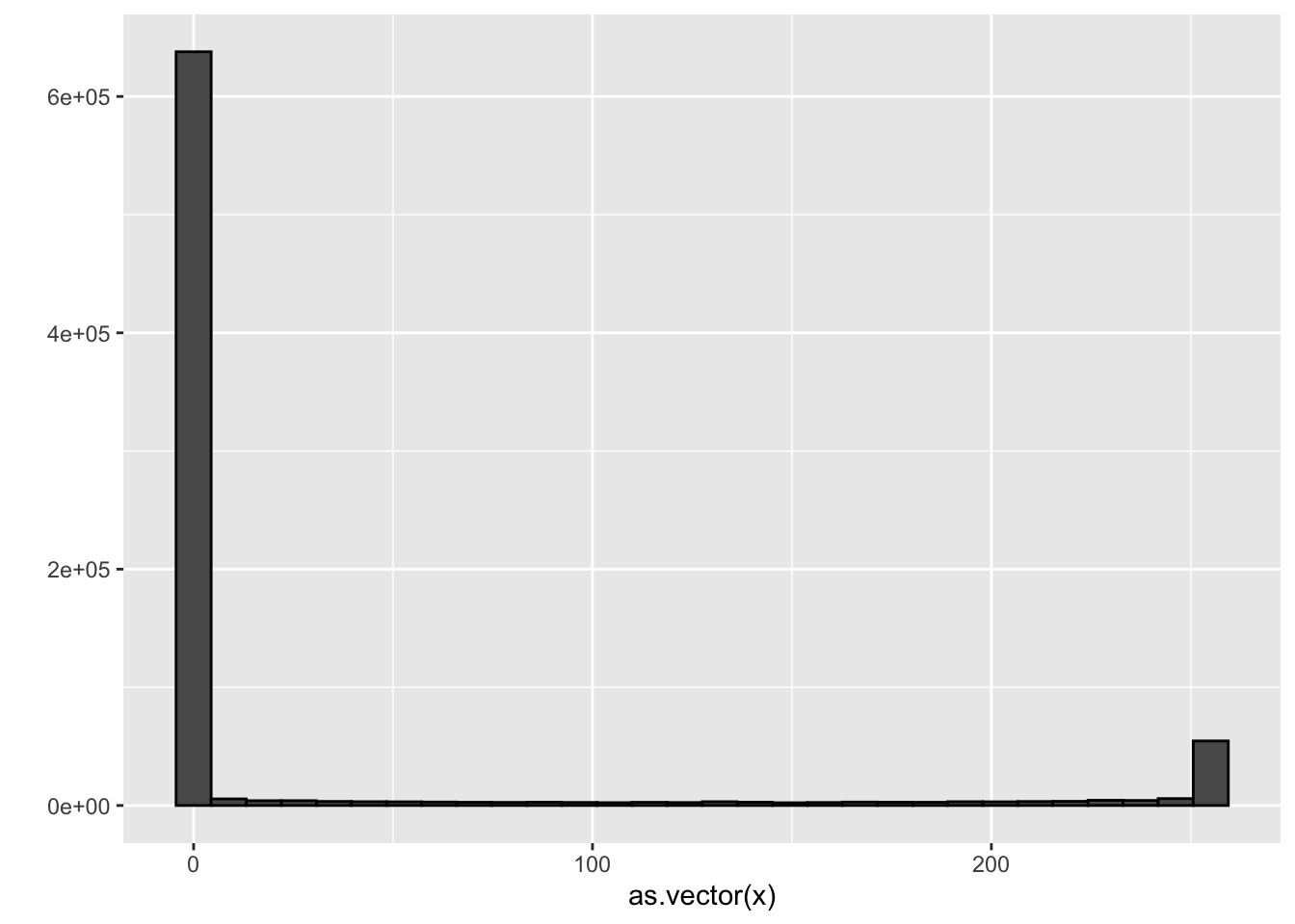

new_x <- x
new_x[new_x < 50] <- 0

mat <- matrix(1:15, 5, 3)
mat[mat < 3] <- 0
mat

##      [,1] [,2] [,3]
## [1,]    0    6   11
## [2,]    0    7   12
## [3,]    3    8   13
## [4,]    4    9   14
## [5,]    5   10   15

mat <- matrix(1:15, 5, 3)
mat[mat > 6 & mat < 12] <- 0
mat

##      [,1] [,2] [,3]
## [1,]    1    6    0
## [2,]    2    0   12
## [3,]    3    0   13
## [4,]    4    0   14
## [5,]    5    0   15

#binarize the data
bin_x <- x
bin_x[bin_x < 255/2] <- 0
bin_x[bin_x > 255/2] <- 1
bin_X <- (x > 255/2)*1

4.18 Vectorization for Matrices and Matrix Algebra Operations

There is a link to the relevant sections of the textbook: Vectorization for matrices and Matrix algebra operations

Key points

• We can scale each row of a matrix using this line of code:

(x - rowMeans(x)) / rowSds(x)

• To scale each column of a matrix, we use this code:

t(t(X) - colMeans(X))

• We can also use a function called sweep() that works similarly to apply(). It takes each entry of a vector and subtracts it from the corresponding row or column:

X_mean_0 <- sweep(x, 2, colMeans(x))

• Matrix multiplication: t(x) %*% x
• The cross product: crossprod(x)
• The inverse of a function: solve(crossprod(x))
• The QR decomposition: qr(x)

Code

#scale each row of a matrix
(x - rowMeans(x)) / rowSds(x)

#scale each column
t(t(x) - colMeans(x))

#take each entry of a vector and subtracts it from the corresponding row or column
x_mean_0 <- sweep(x, 2, colMeans(x))

#divide by the standard deviation
x_mean_0 <- sweep(x, 2, colMeans(x))
x_standardized <- sweep(x_mean_0, 2, colSds(x), FUN = "/")

4.19 Comprehension Check - Working with Matrices

1. Which line of code correctly creates a 100 by 10 matrix of randomly generated normal numbers and assigns it to x?

• A. x <- matrix(rnorm(1000), 100, 100)

• B. x <- matrix(rnorm(100*10), 100, 10)

• C. x <- matrix(rnorm(100*10), 10, 10)

• D. x <- matrix(rnorm(100*10), 10, 100)

2. Write the line of code that would give you the specified information about the matrix x that you generated in q1. Do not include any spaces in your line of code.

Dimension of x: dim(x)

Number of rows of x: nrow(x) or dim(x)[1] or length(x[,1])

Number of columns of x: ncol(x) or dim(x)[2] or length(x[1,])

3. Which of the following lines of code would add the scalar 1 to row 1, the scalar 2 to row 2, and so on, for the matrix x? Select ALL that apply.

• A. x <- x + seq(nrow(x))

• B. x <- 1:nrow(x)

• C. x <- sweep(x, 2, 1:nrow(x),"+")

• D. x <- sweep(x, 1, 1:nrow(x),"+")

4. Which of the following lines of code would add the scalar 1 to column 1, the scalar 2 to column 2, and so on, for the matrix x? Select ALL that apply.

• A. x <- 1:ncol(x)

• B. x <- 1:col(x)

• C. x <- sweep(x, 2, 1:ncol(x), FUN = "+")

• D. x <- -x

5. Which code correctly computes the average of each row of x?

• A. mean(x)

• B. rowMedians(x)

• C. sapply(x,mean)

• D. rowSums(x)

• E. rowMeans(x)

Which code correctly computes the average of each column of x?

• A. mean(x)

• B. sapply(x,mean)

• C. colMeans(x)

• D. colMedians(x)

• C. colSums(x)

6. For each observation in the mnist training data, compute the proportion of pixels that are in the grey area, defined as values between 50 and 205 (but not including 50 and 205). (To visualize this, you can make a boxplot by digit class.)

What proportion of the 60000*784 pixels in the mnist training data are in the grey area overall, defined as values between 50 and 205? Report your answer to at least 3 significant digits.

mnist <- read_mnist()
y <- rowMeans(mnist$train$images>50 & mnist$train$images<205)
qplot(as.factor(mnist$train$labels), y, geom = "boxplot")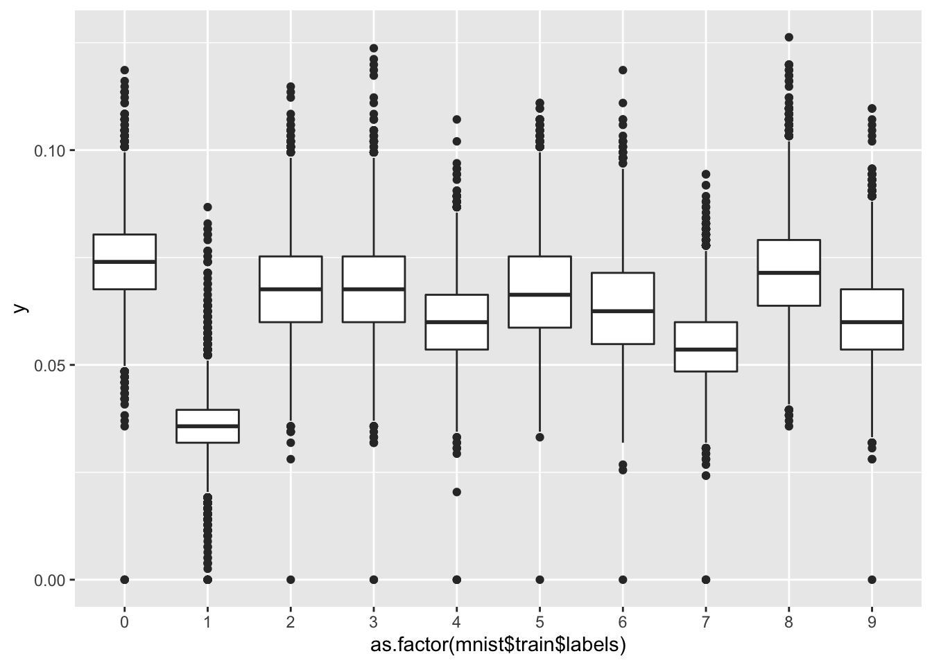

mean(y) # proportion of pixels

## [1] 0.06183703