3 Section 2 Overview
In the Tidy Data section, you will learn how to convert data from a raw to a tidy format.
This section is divided into three parts: Reshaping Data, Combining Tables, and Web Scraping.
After completing the Tidy Data section, you will be able to:
- Reshape data using functions from the tidyr package, including
gather(),spread(),separate(), andunite(). - Combine information from different tables using join functions from the dplyr package.
- Combine information from different tables using binding functions from the dplyr package.
- Use set operators to combine data frames.
- Gather data from a website through web scraping and use of CSS selectors.
3.1 Tidy Data
The textbook for this section is available here.
Key points
- In tidy data, each row represents an observation and each column represents a different variable.
- In wide data, each row includes several observations and one of the variables is stored in the header.
Code
data(gapminder)

# create and inspect a tidy data frame
tidy_data <- gapminder %>%
  filter(country %in% c("South Korea", "Germany")) %>%
  select(country, year, fertility)
head(tidy_data)
## country year fertility
## 1 Germany 1960 2.41
## 2 South Korea 1960 6.16
## 3 Germany 1961 2.44
## 4 South Korea 1961 5.99
## 5 Germany 1962 2.47
## 6 South Korea 1962 5.79# plotting tidy data is simple
tidy_data %>%
ggplot(aes(year, fertility, color = country)) +
geom_point()## Warning: Removed 2 rows containing missing values (geom_point).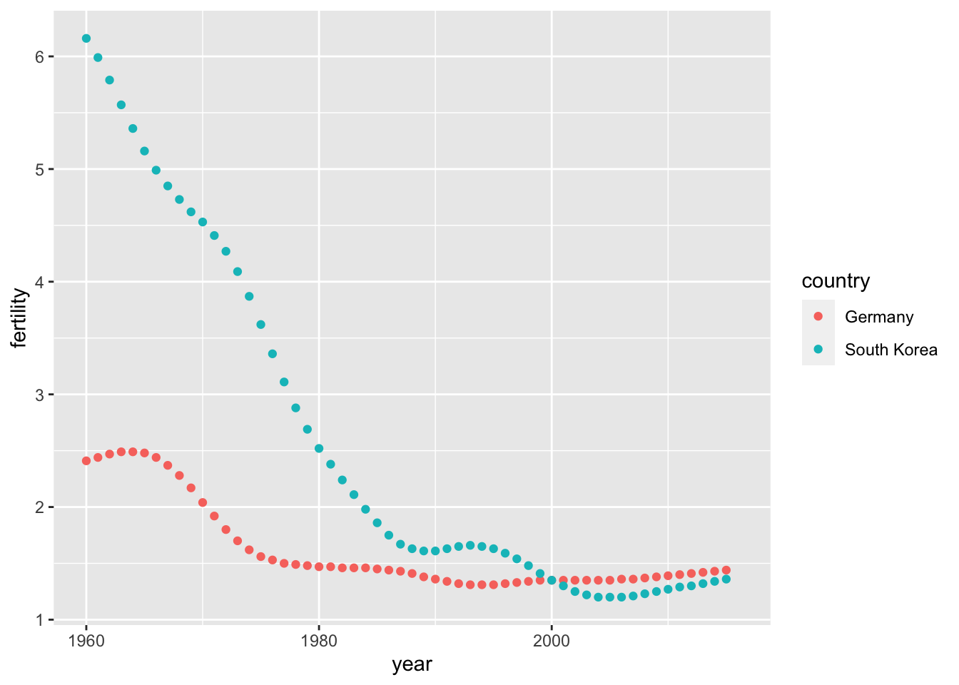
# import and inspect example of original Gapminder data in wide format
path <- system.file("extdata", package="dslabs")
filename <- file.path(path,  "fertility-two-countries-example.csv")
wide_data <- read_csv(filename)
## Parsed with column specification:
## cols(
## .default = col_double(),
## country = col_character()
## )## See spec(...) for full column specifications.select(wide_data, country, `1960`:`1967`)## # A tibble: 2 x 9
## country `1960` `1961` `1962` `1963` `1964` `1965` `1966` `1967`
## <chr> <dbl> <dbl> <dbl> <dbl> <dbl> <dbl> <dbl> <dbl>
## 1 Germany 2.41 2.44 2.47 2.49 2.49 2.48 2.44 2.37
## 2 South Korea 6.16 5.99 5.79 5.57 5.36 5.16 4.99 4.853.2 Reshaping Data
The textbook for this section is available here, here and here.
Key points
- The tidyr package includes several functions that are useful for tidying data.
- The
gather()function converts wide data into tidy data. - The
spread()function converts tidy data to wide data.
Code
# original wide data
path <- system.file("extdata", package="dslabs")
filename <- file.path(path,  "fertility-two-countries-example.csv")
wide_data <- read_csv(filename)
## Parsed with column specification:
## cols(
## .default = col_double(),
## country = col_character()
## )## See spec(...) for full column specifications.# tidy data from dslabs
tidy_data <- gapminder %>%
filter(country %in% c("South Korea", "Germany")) %>%
select(country, year, fertility)
# gather wide data to make new tidy data
new_tidy_data <- wide_data %>%
gather(year, fertility, `1960`:`2015`)
head(new_tidy_data)## # A tibble: 6 x 3
## country year fertility
## <chr> <chr> <dbl>
## 1 Germany 1960 2.41
## 2 South Korea 1960 6.16
## 3 Germany 1961 2.44
## 4 South Korea 1961 5.99
## 5 Germany 1962 2.47
## 6 South Korea 1962 5.79# gather all columns except country
new_tidy_data <- wide_data %>%
gather(year, fertility, -country)
# gather treats column names as characters by default
class(tidy_data$year)## [1] "integer"class(new_tidy_data$year)## [1] "character"# convert gathered column names to numeric
new_tidy_data <- wide_data %>%
gather(year, fertility, -country, convert = TRUE)
class(new_tidy_data$year)## [1] "integer"# ggplot works on new tidy data
new_tidy_data %>%
ggplot(aes(year, fertility, color = country)) +
geom_point()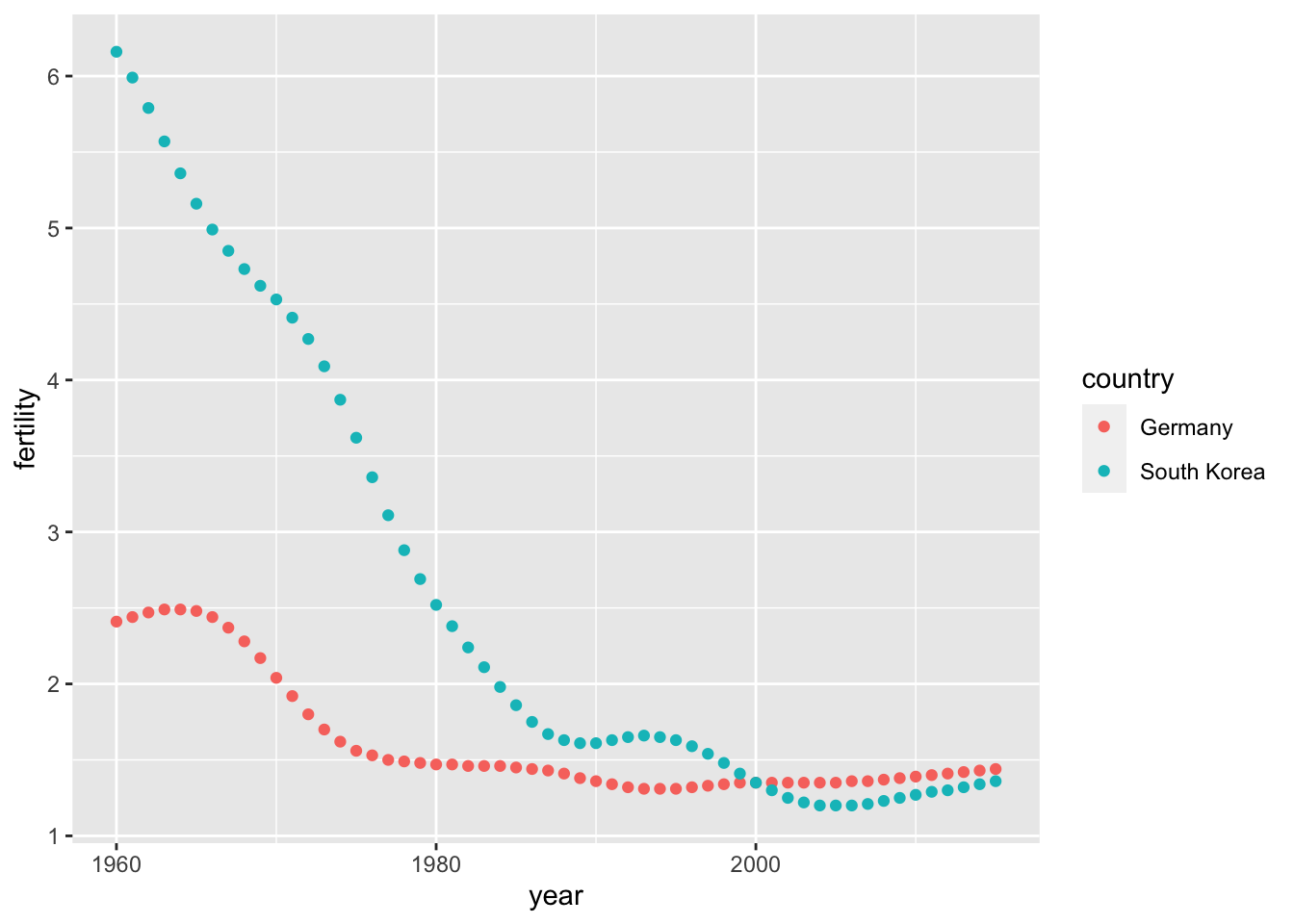
# spread tidy data to generate wide data
new_wide_data <- new_tidy_data %>% spread(year, fertility)
select(new_wide_data, country, `1960`:`1967`)
## # A tibble: 2 x 9
## country `1960` `1961` `1962` `1963` `1964` `1965` `1966` `1967`
## <chr> <dbl> <dbl> <dbl> <dbl> <dbl> <dbl> <dbl> <dbl>
## 1 Germany 2.41 2.44 2.47 2.49 2.49 2.48 2.44 2.37
## 2 South Korea 6.16 5.99 5.79 5.57 5.36 5.16 4.99 4.853.3 Separate and Unite
The textbook for this section is available here and here.
Key points
- The
separate()function splits one column into two or more columns at a specified character that separates the variables. - When there is an extra separation in some of the entries, use
fill="right"to pad missing values with NAs, or useextra="merge"to keep extra elements together. - The
unite()function combines two columns and adds a separating character.
Code
# import data
path <- system.file("extdata", package = "dslabs")
filename <- file.path(path, "life-expectancy-and-fertility-two-countries-example.csv")
raw_dat <- read_csv(filename)
## Parsed with column specification:
## cols(
## .default = col_double(),
## country = col_character()
## )## See spec(...) for full column specifications.select(raw_dat, 1:5)## # A tibble: 2 x 5
## country `1960_fertility` `1960_life_expectancy` `1961_fertility` `1961_life_expectancy`
## <chr> <dbl> <dbl> <dbl> <dbl>
## 1 Germany 2.41 69.3 2.44 69.8
## 2 South Korea 6.16 53.0 5.99 53.8# gather all columns except country
dat <- raw_dat %>% gather(key, value, -country)
head(dat)## # A tibble: 6 x 3
## country key value
## <chr> <chr> <dbl>
## 1 Germany 1960_fertility 2.41
## 2 South Korea 1960_fertility 6.16
## 3 Germany 1960_life_expectancy 69.3
## 4 South Korea 1960_life_expectancy 53.0
## 5 Germany 1961_fertility 2.44
## 6 South Korea 1961_fertility 5.99dat$key[1:5]## [1] "1960_fertility" "1960_fertility" "1960_life_expectancy" "1960_life_expectancy" "1961_fertility"# separate on underscores
dat %>% separate(key, c("year", "variable_name"), "_")## Warning: Expected 2 pieces. Additional pieces discarded in 112 rows [3, 4, 7, 8, 11, 12, 15, 16, 19, 20, 23, 24, 27, 28, 31, 32, 35, 36, 39, 40, ...].## # A tibble: 224 x 4
## country year variable_name value
## <chr> <chr> <chr> <dbl>
## 1 Germany 1960 fertility 2.41
## 2 South Korea 1960 fertility 6.16
## 3 Germany 1960 life 69.3
## 4 South Korea 1960 life 53.0
## 5 Germany 1961 fertility 2.44
## 6 South Korea 1961 fertility 5.99
## 7 Germany 1961 life 69.8
## 8 South Korea 1961 life 53.8
## 9 Germany 1962 fertility 2.47
## 10 South Korea 1962 fertility 5.79
## # … with 214 more rowsdat %>% separate(key, c("year", "variable_name"))## Warning: Expected 2 pieces. Additional pieces discarded in 112 rows [3, 4, 7, 8, 11, 12, 15, 16, 19, 20, 23, 24, 27, 28, 31, 32, 35, 36, 39, 40, ...].## # A tibble: 224 x 4
## country year variable_name value
## <chr> <chr> <chr> <dbl>
## 1 Germany 1960 fertility 2.41
## 2 South Korea 1960 fertility 6.16
## 3 Germany 1960 life 69.3
## 4 South Korea 1960 life 53.0
## 5 Germany 1961 fertility 2.44
## 6 South Korea 1961 fertility 5.99
## 7 Germany 1961 life 69.8
## 8 South Korea 1961 life 53.8
## 9 Germany 1962 fertility 2.47
## 10 South Korea 1962 fertility 5.79
## # … with 214 more rows# split on all underscores, pad empty cells with NA
dat %>% separate(key, c("year", "first_variable_name", "second_variable_name"),
fill = "right")## # A tibble: 224 x 5
## country year first_variable_name second_variable_name value
## <chr> <chr> <chr> <chr> <dbl>
## 1 Germany 1960 fertility <NA> 2.41
## 2 South Korea 1960 fertility <NA> 6.16
## 3 Germany 1960 life expectancy 69.3
## 4 South Korea 1960 life expectancy 53.0
## 5 Germany 1961 fertility <NA> 2.44
## 6 South Korea 1961 fertility <NA> 5.99
## 7 Germany 1961 life expectancy 69.8
## 8 South Korea 1961 life expectancy 53.8
## 9 Germany 1962 fertility <NA> 2.47
## 10 South Korea 1962 fertility <NA> 5.79
## # … with 214 more rows# split on first underscore but keep life_expectancy merged
dat %>% separate(key, c("year", "variable_name"), sep = "_", extra = "merge")## # A tibble: 224 x 4
## country year variable_name value
## <chr> <chr> <chr> <dbl>
## 1 Germany 1960 fertility 2.41
## 2 South Korea 1960 fertility 6.16
## 3 Germany 1960 life_expectancy 69.3
## 4 South Korea 1960 life_expectancy 53.0
## 5 Germany 1961 fertility 2.44
## 6 South Korea 1961 fertility 5.99
## 7 Germany 1961 life_expectancy 69.8
## 8 South Korea 1961 life_expectancy 53.8
## 9 Germany 1962 fertility 2.47
## 10 South Korea 1962 fertility 5.79
## # … with 214 more rows# separate then spread
dat %>% separate(key, c("year", "variable_name"), sep = "_", extra = "merge") %>%
spread(variable_name, value) ## # A tibble: 112 x 4
## country year fertility life_expectancy
## <chr> <chr> <dbl> <dbl>
## 1 Germany 1960 2.41 69.3
## 2 Germany 1961 2.44 69.8
## 3 Germany 1962 2.47 70.0
## 4 Germany 1963 2.49 70.1
## 5 Germany 1964 2.49 70.7
## 6 Germany 1965 2.48 70.6
## 7 Germany 1966 2.44 70.8
## 8 Germany 1967 2.37 71.0
## 9 Germany 1968 2.28 70.6
## 10 Germany 1969 2.17 70.5
## # … with 102 more rows# separate then unite
dat %>%
separate(key, c("year", "first_variable_name", "second_variable_name"), fill = "right") %>%
unite(variable_name, first_variable_name, second_variable_name, sep="_")## # A tibble: 224 x 4
## country year variable_name value
## <chr> <chr> <chr> <dbl>
## 1 Germany 1960 fertility_NA 2.41
## 2 South Korea 1960 fertility_NA 6.16
## 3 Germany 1960 life_expectancy 69.3
## 4 South Korea 1960 life_expectancy 53.0
## 5 Germany 1961 fertility_NA 2.44
## 6 South Korea 1961 fertility_NA 5.99
## 7 Germany 1961 life_expectancy 69.8
## 8 South Korea 1961 life_expectancy 53.8
## 9 Germany 1962 fertility_NA 2.47
## 10 South Korea 1962 fertility_NA 5.79
## # … with 214 more rows# full code for tidying data
dat %>%
separate(key, c("year", "first_variable_name", "second_variable_name"), fill = "right") %>%
unite(variable_name, first_variable_name, second_variable_name, sep="_") %>%
spread(variable_name, value) %>%
rename(fertility = fertility_NA)## # A tibble: 112 x 4
## country year fertility life_expectancy
## <chr> <chr> <dbl> <dbl>
## 1 Germany 1960 2.41 69.3
## 2 Germany 1961 2.44 69.8
## 3 Germany 1962 2.47 70.0
## 4 Germany 1963 2.49 70.1
## 5 Germany 1964 2.49 70.7
## 6 Germany 1965 2.48 70.6
## 7 Germany 1966 2.44 70.8
## 8 Germany 1967 2.37 71.0
## 9 Germany 1968 2.28 70.6
## 10 Germany 1969 2.17 70.5
## # … with 102 more rows3.4 Assessment Part 1 - Reshaping Data
- A collaborator sends you a file containing data for three years of average race finish times.
age_group,2015,2016,2017
20,3:46,3:22,3:50
30,3:50,3:43,4:43
40,4:39,3:49,4:51
50,4:48,4:59,5:01
Are these data considered “tidy” in R? Why or why not?
- A. Yes. These data are considered “tidy” because each row contains unique observations.
- B. Yes. These data are considered “tidy” because there are no missing data in the data frame.
- C. No. These data are not considered “tidy” because the variable “year” is stored in the header.
- D. No. These data are not considered “tidy” because there are not an equal number of columns and rows.
- Below are four versions of the same dataset. Which one is in a tidy format?
- A.
state      abb   region  population total
Alabama    AL    South   4779736    135
Alaska     AK    West    710231     19
Arizona    AZ    West    6392017    232
Arkansas   AR    South   2915918    93
California CA    West    37253956   1257
Colorado CO West 5029196 65- B.
state    abb  region        var        people
Alabama  AL   South         population 4779736
Alabama  AL   South         total      135
Alaska   AK   West          population 710231
Alaska   AK   West          total      19
Arizona  AZ   West          population 6392017
Arizona AZ West total 232- C.
state       abb       Northeast   South      North Central   West
Alabama     AL        NA          4779736    NA              NA
Alaska      AK        NA          NA         NA              710231
Arizona     AZ        NA          NA         NA              6392017
Arkansas    AR        NA          2915918    NA              NA
California  CA        NA          NA         NA              37253956
Colorado CO NA NA NA 5029196- D.
state       abb  region    rate
Alabama     AL   South     2.82e-05
Alaska      AK   West      2.68e-05
Arizona     AZ   West      3.63e-05
Arkansas    AR   South     3.19e-05
California  CA   West      3.37e-05
Colorado CO West 1.29e-05- Your file called “times.csv” has age groups and average race finish times for three years of marathons.
age_group,2015,2016,2017
20,3:46,3:22,3:50
30,3:50,3:43,4:43
40,4:39,3:49,4:51
50,4:48,4:59,5:01
You read in the data file using the following command.
d <- read_csv("files/times.csv")## Parsed with column specification:
## cols(
## age_group = col_double(),
## `2015` = col_time(format = ""),
## `2016` = col_time(format = ""),
## `2017` = col_time(format = "")
## )Which commands will help you “tidy” the data?
tidy_data <- d %>%
gather(year, time, `2015`:`2017`)
tidy_data
## # A tibble: 12 x 3
## age_group year time
## <dbl> <chr> <time>
## 1 20 2015 03:46
## 2 30 2015 03:50
## 3 40 2015 04:39
## 4 50 2015 04:48
## 5 20 2016 03:22
## 6 30 2016 03:43
## 7 40 2016 03:49
## 8 50 2016 04:59
## 9 20 2017 03:50
## 10 30 2017 04:43
## 11 40 2017 04:51
## 12 50 2017 05:01- A.
tidy_data <- d %>%
gather(year, time, `2015`:`2017`)- B.
tidy_data <- d %>%
spread(year, time, `2015`:`2017`)- C.
tidy_data <- d %>%
gather(age_group, year, time, `2015`:`2017`)- D.
tidy_data <- d %>%
gather(time, `2015`:`2017`)- You have a dataset on U.S. contagious diseases, but it is in the following wide format:
> head(dat_wide)
state   year    population      Hepatitis A Mumps Polio Rubella
Alabama 1990    4040587         86          19    76    1
Alabama 1991    4066003         39          14    65    0
Alabama 1992    4097169         35          12    24    0
Alabama 1993    4133242         40          22    67    0
Alabama 1994    4173361         72          12    39    0
Alabama 1995    4216645         75          2     38    0
Which of the following would transform this into a tidy dataset, with each row representing an observation of the incidence of each specific disease (as shown below)?
> head(dat_tidy)
state   year    population   disease      count
Alabama 1990    4040587      Hepatitis A  86
Alabama 1991    4066003      Hepatitis A  39
Alabama 1992    4097169      Hepatitis A  35
Alabama 1993    4133242      Hepatitis A  40
Alabama 1994    4173361      Hepatitis A  72
Alabama 1995 4216645 Hepatitis A 75- A.
dat_tidy <- dat_wide %>%
gather (key = count, value = disease, `Hepatitis A`, `Rubella`)- B.
dat_tidy <- dat_wide %>%
gather(key = count, value = disease, -state, -year, -population)- C.
dat_tidy <- dat_wide %>%
gather(key = disease, value = count, -state)- D.
dat_tidy <- dat_wide %>%
gather(key = disease, value = count, “Hepatitis A”: “Rubella”)- You have successfully formatted marathon finish times into a tidy object called
tidy_data. The first few lines are shown below.
age_group year  time
20        2015  03:46
30        2015  03:50
40        2015  04:39
50        2015  04:48
20        2016  03:22
Select the code that converts these data back to the wide format, where each year has a separate column.
tidy_data %>% spread(year, time)## # A tibble: 4 x 4
## age_group `2015` `2016` `2017`
## <dbl> <time> <time> <time>
## 1 20 03:46 03:22 03:50
## 2 30 03:50 03:43 04:43
## 3 40 04:39 03:49 04:51
## 4 50 04:48 04:59 05:01-
A.
tidy_data %>% spread(time, year) -
B.
tidy_data %>% spread(year, time) -
C.
tidy_data %>% spread(year, age_group) -
D.
tidy_data %>% spread(time, year, `2015`:`2017`)
- You have the following dataset:
> head(dat)
state    abb  region        var         people
Alabama  AL   South         population  4779736
Alabama  AL   South         total       135
Alaska   AK   West          population  710231
Alaska   AK   West          total       19
Arizona  AZ   West          population  6392017
Arizona  AZ   West          total       232
You would like to transform it into a dataset where population and total are each their own column (shown below). Which code would best accomplish this?
state       abb  region  population total
Alabama     AL   South   4779736    135
Alaska      AK   West    710231     19
Arizona     AZ   West    6392017    232
Arkansas    AR   South   2915918    93
California  CA   West    37253956   1257
Colorado CO West 5029196 65-
A.
dat_tidy <- dat %>% spread(key = var, value = people) -
B.
dat_tidy <- dat %>% spread(key = state:region, value = people) -
C.
dat_tidy <- dat %>% spread(key = people, value = var) -
D.
dat_tidy <- dat %>% spread(key = region, value = people)
- A collaborator sends you a file containing data for two years of average race finish times, “times2.csv”:.
age_group,2015_time,2015_participants,2016_time,2016_participants
20,3:46,54,3:22,62
30,3:50,60,3:43,58
40,4:39,29,3:49,33
50,4:48,10,4:59,14
You read in the data file
d <- read_csv("files/times2.csv")## Parsed with column specification:
## cols(
## age_group = col_double(),
## `2015_time` = col_time(format = ""),
## `2015_participants` = col_double(),
## `2016_time` = col_time(format = ""),
## `2016_participants` = col_double()
## )Which of the answers below best tidys the data?
tidy_data <- d %>%
        gather(key = "key", value = "value", -age_group) %>%
    separate(col = key, into = c("year", "variable_name"), sep = "_") %>%
    spread(key = variable_name, value = value)
## Warning: attributes are not identical across measure variables;
## they will be droppedtidy_data## # A tibble: 8 x 4
## age_group year participants time
## <dbl> <chr> <dbl> <dbl>
## 1 20 2015 54 13560
## 2 20 2016 62 12120
## 3 30 2015 60 13800
## 4 30 2016 58 13380
## 5 40 2015 29 16740
## 6 40 2016 33 13740
## 7 50 2015 10 17280
## 8 50 2016 14 17940- A.
tidy_data <- d %>%
    gather(key = “key”, value = “value”, -age_group) %>%
    separate(col = key, into = c(“year”, “variable_name”), sep = “.”) %>%
spread(key = variable_name, value = value)- B.
tidy_data <- d %>%
        gather(key = “key”, value = “value”, -age_group) %>%
    separate(col = key, into = c(“year”, “variable_name”), sep = “_”) %>%
spread(key = variable_name, value = value)- C.
 tidy_data <- d %>%
        gather(key = “key”, value = “value”) %>%
    separate(col = key, into = c(“year”, “variable_name”), sep = “_”) %>%
spread(key = variable_name, value = value)- D.
tidy_data <- d %>%
        gather(key = “key”, value = “value”, -age_group) %>%
    separate(col = key, into = “year”, sep = “_”) %>%
spread(key = year, value = value)- You are in the process of tidying some data on heights, hand length, and wingspan for basketball players in the draft. Currently, you have the following:
> head(stats)
key                 value
allen_height        75
allen_hand_length   8.25
allen_wingspan      79.25
bamba_height        83.25
bamba_hand_length   9.75
bamba_wingspan      94
Select all of the correct commands below that would turn this data into a “tidy” format.
- A.
tidy_data <- stats %>%
    separate(col = key, into = c("player", "variable_name"), sep = "_", extra = "merge") %>%
spread(key = variable_name, value = value) - B.
tidy_data <- stats %>%
    separate(col = key, into = c("player", "variable_name1", "variable_name2"), sep = "_", fill = "right") %>%
    unite(col = variable_name, variable_name1, variable_name2, sep = "_") %>%
spread(key = variable_name, value = value)- C.
tidy_data <- stats %>%
    separate(col = key, into = c("player", "variable_name"), sep = "_") %>%
    spread(key = variable_name, value = value)
3.5 Assessment Part 2 - Reshaping Data
- Examine the built-in dataset
co2. This dataset comes with base R, not dslabs - just typeco2to access the dataset.
co2## Jan Feb Mar Apr May Jun Jul Aug Sep Oct Nov Dec
## 1959 315.42 316.31 316.50 317.56 318.13 318.00 316.39 314.65 313.68 313.18 314.66 315.43
## 1960 316.27 316.81 317.42 318.87 319.87 319.43 318.01 315.74 314.00 313.68 314.84 316.03
## 1961 316.73 317.54 318.38 319.31 320.42 319.61 318.42 316.63 314.83 315.16 315.94 316.85
## 1962 317.78 318.40 319.53 320.42 320.85 320.45 319.45 317.25 316.11 315.27 316.53 317.53
## 1963 318.58 318.92 319.70 321.22 322.08 321.31 319.58 317.61 316.05 315.83 316.91 318.20
## 1964 319.41 320.07 320.74 321.40 322.06 321.73 320.27 318.54 316.54 316.71 317.53 318.55
## 1965 319.27 320.28 320.73 321.97 322.00 321.71 321.05 318.71 317.66 317.14 318.70 319.25
## 1966 320.46 321.43 322.23 323.54 323.91 323.59 322.24 320.20 318.48 317.94 319.63 320.87
## 1967 322.17 322.34 322.88 324.25 324.83 323.93 322.38 320.76 319.10 319.24 320.56 321.80
## 1968 322.40 322.99 323.73 324.86 325.40 325.20 323.98 321.95 320.18 320.09 321.16 322.74
## 1969 323.83 324.26 325.47 326.50 327.21 326.54 325.72 323.50 322.22 321.62 322.69 323.95
## 1970 324.89 325.82 326.77 327.97 327.91 327.50 326.18 324.53 322.93 322.90 323.85 324.96
## 1971 326.01 326.51 327.01 327.62 328.76 328.40 327.20 325.27 323.20 323.40 324.63 325.85
## 1972 326.60 327.47 327.58 329.56 329.90 328.92 327.88 326.16 324.68 325.04 326.34 327.39
## 1973 328.37 329.40 330.14 331.33 332.31 331.90 330.70 329.15 327.35 327.02 327.99 328.48
## 1974 329.18 330.55 331.32 332.48 332.92 332.08 331.01 329.23 327.27 327.21 328.29 329.41
## 1975 330.23 331.25 331.87 333.14 333.80 333.43 331.73 329.90 328.40 328.17 329.32 330.59
## 1976 331.58 332.39 333.33 334.41 334.71 334.17 332.89 330.77 329.14 328.78 330.14 331.52
## 1977 332.75 333.24 334.53 335.90 336.57 336.10 334.76 332.59 331.42 330.98 332.24 333.68
## 1978 334.80 335.22 336.47 337.59 337.84 337.72 336.37 334.51 332.60 332.38 333.75 334.78
## 1979 336.05 336.59 337.79 338.71 339.30 339.12 337.56 335.92 333.75 333.70 335.12 336.56
## 1980 337.84 338.19 339.91 340.60 341.29 341.00 339.39 337.43 335.72 335.84 336.93 338.04
## 1981 339.06 340.30 341.21 342.33 342.74 342.08 340.32 338.26 336.52 336.68 338.19 339.44
## 1982 340.57 341.44 342.53 343.39 343.96 343.18 341.88 339.65 337.81 337.69 339.09 340.32
## 1983 341.20 342.35 342.93 344.77 345.58 345.14 343.81 342.21 339.69 339.82 340.98 342.82
## 1984 343.52 344.33 345.11 346.88 347.25 346.62 345.22 343.11 340.90 341.18 342.80 344.04
## 1985 344.79 345.82 347.25 348.17 348.74 348.07 346.38 344.51 342.92 342.62 344.06 345.38
## 1986 346.11 346.78 347.68 349.37 350.03 349.37 347.76 345.73 344.68 343.99 345.48 346.72
## 1987 347.84 348.29 349.23 350.80 351.66 351.07 349.33 347.92 346.27 346.18 347.64 348.78
## 1988 350.25 351.54 352.05 353.41 354.04 353.62 352.22 350.27 348.55 348.72 349.91 351.18
## 1989 352.60 352.92 353.53 355.26 355.52 354.97 353.75 351.52 349.64 349.83 351.14 352.37
## 1990 353.50 354.55 355.23 356.04 357.00 356.07 354.67 352.76 350.82 351.04 352.69 354.07
## 1991 354.59 355.63 357.03 358.48 359.22 358.12 356.06 353.92 352.05 352.11 353.64 354.89
## 1992 355.88 356.63 357.72 359.07 359.58 359.17 356.94 354.92 352.94 353.23 354.09 355.33
## 1993 356.63 357.10 358.32 359.41 360.23 359.55 357.53 355.48 353.67 353.95 355.30 356.78
## 1994 358.34 358.89 359.95 361.25 361.67 360.94 359.55 357.49 355.84 356.00 357.59 359.05
## 1995 359.98 361.03 361.66 363.48 363.82 363.30 361.94 359.50 358.11 357.80 359.61 360.74
## 1996 362.09 363.29 364.06 364.76 365.45 365.01 363.70 361.54 359.51 359.65 360.80 362.38
## 1997 363.23 364.06 364.61 366.40 366.84 365.68 364.52 362.57 360.24 360.83 362.49 364.34Is co2 tidy? Why or why not?
-
A.
co2is tidy data: it has one year for each row. -
B.
co2is tidy data: each column is a different month. -
C.
co2is not tidy: there are multiple observations per column. -
D.
co2is not tidy: to be tidy we would have to wrangle it to have three columns (year, month and value), and then each co2 observation would have a row.
- Run the following command to define the co2_wide object:
co2_wide <- data.frame(matrix(co2, ncol = 12, byrow = TRUE)) %>%
      setNames(1:12) %>%
    mutate(year = as.character(1959:1997))
Use the gather() function to make this dataset tidy. Call the column with the CO2 measurements co2 and call the month column month. Name the resulting object co2_tidy.
Which code would return the correct tidy format?
co2_tidy <- gather(co2_wide,month,co2,-year)-
A.
co2_tidy <- gather(co2_wide,month,co2,year) -
B.
co2_tidy <- gather(co2_wide,co2,month,-year) -
C.
co2_tidy <- gather(co2_wide,co2,month,year) -
D.
co2_tidy <- gather(co2_wide,month,co2,-year)
- Use
co2_tidyto plot CO2 versus month with a different curve for each year:
co2_tidy %>% ggplot(aes(as.numeric(month), co2, color = year)) + geom_line()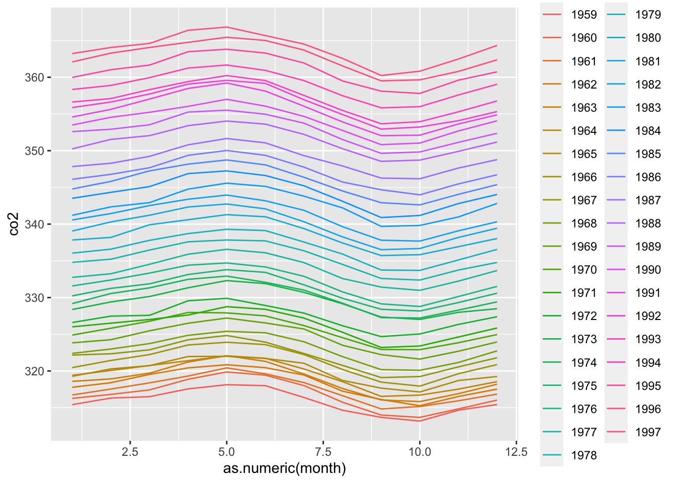
What can be concluded from this plot?
- A. CO2 concentrations increased monotonically (never decreased) from 1959 to 1997.
- B. CO2 concentrations are highest around May and the yearly average increased from 1959 to 1997.
- C. CO2 concentrations are highest around October and the yearly average increased from 1959 to 1997.
- D. Yearly average CO2 concentrations have remained constant over time.
- E. CO2 concentrations do not have a seasonal trend.
- Load the
admissionsdataset from dslabs, which contains college admission information for men and women across six majors, and remove theapplicantspercentage column:
data(admissions)
dat <- admissions %>% select(-applicants)
Your goal is to get the data in the shape that has one row for each major, like this:
major  men   women
A      62    82
B      63    68
C      37    34
D      33    35
E      28    24
F       6     7
Which command could help you to wrangle the data into the desired format?
dat_tidy <- spread(dat, gender, admitted)-
A.
dat_tidy <- spread(dat, major, admitted) -
B.
dat_tidy <- spread(dat, gender, major) -
C.
dat_tidy <- spread(dat, gender, admitted) -
D.
dat_tidy <- spread(dat, admitted, gender)
- Now use the
admissionsdataset to create the objecttmp, which has columnsmajor,gender,keyandvalue:
tmp <- gather(admissions, key, value, admitted:applicants)
tmp
## major gender key value
## 1 A men admitted 62
## 2 B men admitted 63
## 3 C men admitted 37
## 4 D men admitted 33
## 5 E men admitted 28
## 6 F men admitted 6
## 7 A women admitted 82
## 8 B women admitted 68
## 9 C women admitted 34
## 10 D women admitted 35
## 11 E women admitted 24
## 12 F women admitted 7
## 13 A men applicants 825
## 14 B men applicants 560
## 15 C men applicants 325
## 16 D men applicants 417
## 17 E men applicants 191
## 18 F men applicants 373
## 19 A women applicants 108
## 20 B women applicants 25
## 21 C women applicants 593
## 22 D women applicants 375
## 23 E women applicants 393
## 24 F women applicants 341Combine the key and gender and create a new column called column_name to get a variable with the following values: admitted_men, admitted_women, applicants_menand applicants_women. Save the new data as tmp2.
Which command could help you to wrangle the data into the desired format?
tmp2 <- unite(tmp, column_name, c(key, gender))-
A.
tmp2 <- spread(tmp, column_name, key, gender) -
B.
tmp2 <- gather(tmp, column_name, c(gender,key)) -
C.
tmp2 <- unite(tmp, column_name, c(gender, key)) -
D.
tmp2 <- spread(tmp, column_name, c(key,gender)) -
E.
tmp2 <- unite(tmp, column_name, c(key, gender))
- Which function can reshape
tmp2to a table with six rows and five columns namedmajor,admitted_men,admitted_women,applicants_menandapplicants_women?
spread(tmp2, column_name, value)## major admitted_men admitted_women applicants_men applicants_women
## 1 A 62 82 825 108
## 2 B 63 68 560 25
## 3 C 37 34 325 593
## 4 D 33 35 417 375
## 5 E 28 24 191 393
## 6 F 6 7 373 341-
A.
gather() -
B.
spread() -
C.
separate() -
D.
unite()
3.6 Combining Tables
The textbook for this section is available here.
Key points
- The join functions in the dplyr package combine two tables such that matching rows are together.
left_join()only keeps rows that have information in the first table.right_join()only keeps rows that have information in the second table.inner_join()only keeps rows that have information in both tables.full_join()keeps all rows from both tables.semi_join()keeps the part of first table for which we have information in the second.anti_join()keeps the elements of the first table for which there is no information in the second.
Code
if(!require(ggrepel)) install.packages("ggrepel")## Loading required package: ggrepel# import US murders data
library(ggrepel)
ds_theme_set()
data(murders)
head(murders)## state abb region population total
## 1 Alabama AL South 4779736 135
## 2 Alaska AK West 710231 19
## 3 Arizona AZ West 6392017 232
## 4 Arkansas AR South 2915918 93
## 5 California CA West 37253956 1257
## 6 Colorado CO West 5029196 65# import US election results data
data(polls_us_election_2016)
head(results_us_election_2016)## state electoral_votes clinton trump others
## 1 California 55 61.7 31.6 6.7
## 2 Texas 38 43.2 52.2 4.5
## 3 Florida 29 47.8 49.0 3.2
## 4 New York 29 59.0 36.5 4.5
## 5 Illinois 20 55.8 38.8 5.4
## 6 Pennsylvania 20 47.9 48.6 3.6identical(results_us_election_2016$state, murders$state)## [1] FALSE# join the murders table and US election results table
tab <- left_join(murders, results_us_election_2016, by = "state")
head(tab)## state abb region population total electoral_votes clinton trump others
## 1 Alabama AL South 4779736 135 9 34.4 62.1 3.6
## 2 Alaska AK West 710231 19 3 36.6 51.3 12.2
## 3 Arizona AZ West 6392017 232 11 45.1 48.7 6.2
## 4 Arkansas AR South 2915918 93 6 33.7 60.6 5.8
## 5 California CA West 37253956 1257 55 61.7 31.6 6.7
## 6 Colorado CO West 5029196 65 9 48.2 43.3 8.6# plot electoral votes versus population
tab %>% ggplot(aes(population/10^6, electoral_votes, label = abb)) +
geom_point() +
geom_text_repel() +
scale_x_continuous(trans = "log2") +
scale_y_continuous(trans = "log2") +
geom_smooth(method = "lm", se = FALSE)## `geom_smooth()` using formula 'y ~ x'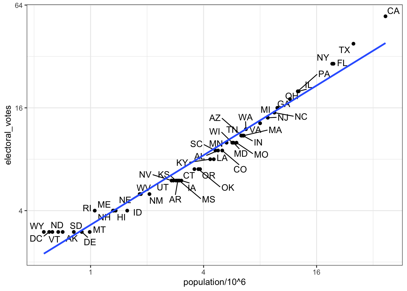
# make two smaller tables to demonstrate joins
tab1 <- slice(murders, 1:6) %>% select(state, population)
tab1
## state population
## 1 Alabama 4779736
## 2 Alaska 710231
## 3 Arizona 6392017
## 4 Arkansas 2915918
## 5 California 37253956
## 6 Colorado 5029196tab2 <- slice(results_us_election_2016, c(1:3, 5, 7:8)) %>% select(state, electoral_votes)
tab2## state electoral_votes
## 1 California 55
## 2 Texas 38
## 3 Florida 29
## 4 Illinois 20
## 5 Ohio 18
## 6 Georgia 16# experiment with different joins
left_join(tab1, tab2)## Joining, by = "state"## state population electoral_votes
## 1 Alabama 4779736 NA
## 2 Alaska 710231 NA
## 3 Arizona 6392017 NA
## 4 Arkansas 2915918 NA
## 5 California 37253956 55
## 6 Colorado 5029196 NAtab1 %>% left_join(tab2)## Joining, by = "state"## state population electoral_votes
## 1 Alabama 4779736 NA
## 2 Alaska 710231 NA
## 3 Arizona 6392017 NA
## 4 Arkansas 2915918 NA
## 5 California 37253956 55
## 6 Colorado 5029196 NAtab1 %>% right_join(tab2)## Joining, by = "state"## state population electoral_votes
## 1 California 37253956 55
## 2 Texas NA 38
## 3 Florida NA 29
## 4 Illinois NA 20
## 5 Ohio NA 18
## 6 Georgia NA 16inner_join(tab1, tab2)## Joining, by = "state"## state population electoral_votes
## 1 California 37253956 55semi_join(tab1, tab2)## Joining, by = "state"## state population
## 1 California 37253956anti_join(tab1, tab2)## Joining, by = "state"## state population
## 1 Alabama 4779736
## 2 Alaska 710231
## 3 Arizona 6392017
## 4 Arkansas 2915918
## 5 Colorado 50291963.7 Binding
The textbook for this section is available here.
Key points
- Unlike the join functions, the binding functions do not try to match by a variable, but rather just combine datasets.
bind_cols()binds two objects by making them columns in a tibble. The R-base functioncbind()binds columns but makes a data frame or matrix instead.- The
bind_rows()function is similar but binds rows instead of columns. The R-base functionrbind()binds rows but makes a data frame or matrix instead.
Code
bind_cols(a = 1:3, b = 4:6)## # A tibble: 3 x 2
## a b
## <int> <int>
## 1 1 4
## 2 2 5
## 3 3 6tab1 <- tab[, 1:3]
tab2 <- tab[, 4:6]
tab3 <- tab[, 7:9]
new_tab <- bind_cols(tab1, tab2, tab3)
head(new_tab)## state abb region population total electoral_votes clinton trump others
## 1 Alabama AL South 4779736 135 9 34.4 62.1 3.6
## 2 Alaska AK West 710231 19 3 36.6 51.3 12.2
## 3 Arizona AZ West 6392017 232 11 45.1 48.7 6.2
## 4 Arkansas AR South 2915918 93 6 33.7 60.6 5.8
## 5 California CA West 37253956 1257 55 61.7 31.6 6.7
## 6 Colorado CO West 5029196 65 9 48.2 43.3 8.6tab1 <- tab[1:2,]
tab2 <- tab[3:4,]
bind_rows(tab1, tab2)## state abb region population total electoral_votes clinton trump others
## 1 Alabama AL South 4779736 135 9 34.4 62.1 3.6
## 2 Alaska AK West 710231 19 3 36.6 51.3 12.2
## 3 Arizona AZ West 6392017 232 11 45.1 48.7 6.2
## 4 Arkansas AR South 2915918 93 6 33.7 60.6 5.83.8 Set Operators
The textbook for this section is available here.
Key points
- By default, the set operators in R-base work on vectors. If tidyverse/dplyr are loaded, they also work on data frames.
- You can take intersections of vectors using
intersect(). This returns the elements common to both sets. - You can take the union of vectors using
union(). This returns the elements that are in either set. - The set difference between a first and second argument can be obtained with
setdiff(). Note that this function is not symmetric. - The function
set_equal()tells us if two sets are the same, regardless of the order of elements.
Code
# intersect vectors or data frames
intersect(1:10, 6:15)
## [1] 6 7 8 9 10intersect(c("a","b","c"), c("b","c","d"))## [1] "b" "c"tab1 <- tab[1:5,]
tab2 <- tab[3:7,]
intersect(tab1, tab2)## state abb region population total electoral_votes clinton trump others
## 1 Arizona AZ West 6392017 232 11 45.1 48.7 6.2
## 2 Arkansas AR South 2915918 93 6 33.7 60.6 5.8
## 3 California CA West 37253956 1257 55 61.7 31.6 6.7# perform a union of vectors or data frames
union(1:10, 6:15)## [1] 1 2 3 4 5 6 7 8 9 10 11 12 13 14 15union(c("a","b","c"), c("b","c","d"))## [1] "a" "b" "c" "d"tab1 <- tab[1:5,]
tab2 <- tab[3:7,]
union(tab1, tab2)## state abb region population total electoral_votes clinton trump others
## 1 Alabama AL South 4779736 135 9 34.4 62.1 3.6
## 2 Alaska AK West 710231 19 3 36.6 51.3 12.2
## 3 Arizona AZ West 6392017 232 11 45.1 48.7 6.2
## 4 Arkansas AR South 2915918 93 6 33.7 60.6 5.8
## 5 California CA West 37253956 1257 55 61.7 31.6 6.7
## 6 Colorado CO West 5029196 65 9 48.2 43.3 8.6
## 7 Connecticut CT Northeast 3574097 97 7 54.6 40.9 4.5# set difference of vectors or data frames
setdiff(1:10, 6:15)## [1] 1 2 3 4 5setdiff(6:15, 1:10)## [1] 11 12 13 14 15tab1 <- tab[1:5,]
tab2 <- tab[3:7,]
setdiff(tab1, tab2)## state abb region population total electoral_votes clinton trump others
## 1 Alabama AL South 4779736 135 9 34.4 62.1 3.6
## 2 Alaska AK West 710231 19 3 36.6 51.3 12.2# setequal determines whether sets have the same elements, regardless of order
setequal(1:5, 1:6)## [1] FALSEsetequal(1:5, 5:1)## [1] TRUEsetequal(tab1, tab2)## [1] FALSE3.9 Assessment - Combining Tables
- You have created a
tab1andtab2of state population and election data:
> tab1
state                    population
Alabama                  4779736
Alaska                   710231
Arizona                  6392017
Delaware                 897934
District of Columbia     601723

> tab2
state        electoral_votes
Alabama      9
Alaska       3
Arizona      11
California   55
Colorado     9
Connecticut  7

> dim(tab1)
[1] 5 2

> dim(tab2)
[1] 6 2
What are the dimensions of the table dat, created by the following command?
dat <- left_join(tab1, tab2, by = “state”)- A. 3 rows by 3 columns
- B. 5 rows by 2 columns
- C. 5 rows by 3 columns
- D. 6 rows by 3 columns
- We are still using the
tab1and ```tab2 tables shown in question 1. What join command would create a new table “dat” with three rows and two columns?
-
A.
dat <- right_join(tab1, tab2, by = “state”) -
B.
dat <- full_join(tab1, tab2, by = “state”) -
C.
dat <- inner_join(tab1, tab2, by = “state”) -
D.
dat <- semi_join(tab1, tab2, by = “state”)
- Which of the following are real differences between the join and bind functions?
- A. Binding functions combine by position, while join functions match by variables.
- B. Joining functions can join datasets of different dimensions, but the bind functions must match on the appropriate dimension (either same row or column numbers).
- C. Bind functions can combine both vectors and dataframes, while join functions work for only for dataframes.
- D. The join functions are a part of the dplyr package and have been optimized for speed, while the bind functions are inefficient base functions.
- We have two simple tables, shown below, with columns
xandy:
> df1
 x     y
 a     a
 b     a

> df2
 x     y
 a     a
 a     b
Which command would result in the following table?
> final
 x     y
b a -
A.
final <- union(df1, df2) -
B.
final <- setdiff(df1, df2) -
C.
final <- setdiff(df2, df1) -
D.
final <- intersect(df1, df2)
Install and load the Lahman library. This library contains a variety of datasets related to US professional baseball. We will use this library for the next few questions and will discuss it more extensively in the Regression course. For now, focus on wrangling the data rather than understanding the statistics.
The Batting data frame contains the offensive statistics for all baseball players over several seasons. Filter this data frame to define top as the top 10 home run (HR) hitters in 2016:
if(!require(Lahman)) install.packages("Lahman")## Loading required package: Lahmanlibrary(Lahman)
top <- Batting %>%
filter(yearID == 2016) %>%
arrange(desc(HR)) %>% # arrange by descending HR count
slice(1:10) # take entries 1-10
top %>% as_tibble()## # A tibble: 10 x 22
## playerID yearID stint teamID lgID G AB R H X2B X3B HR RBI SB CS BB SO IBB HBP SH SF GIDP
## <chr> <int> <int> <fct> <fct> <int> <int> <int> <int> <int> <int> <int> <int> <int> <int> <int> <int> <int> <int> <int> <int> <int>
## 1 trumbma01 2016 1 BAL AL 159 613 94 157 27 1 47 108 2 0 51 170 1 3 0 0 14
## 2 cruzne02 2016 1 SEA AL 155 589 96 169 27 1 43 105 2 0 62 159 5 9 0 7 15
## 3 daviskh01 2016 1 OAK AL 150 555 85 137 24 2 42 102 1 2 42 166 0 8 0 5 19
## 4 doziebr01 2016 1 MIN AL 155 615 104 165 35 5 42 99 18 2 61 138 6 8 2 5 12
## 5 encared01 2016 1 TOR AL 160 601 99 158 34 0 42 127 2 0 87 138 3 5 0 8 22
## 6 arenano01 2016 1 COL NL 160 618 116 182 35 6 41 133 2 3 68 103 10 2 0 8 17
## 7 cartech02 2016 1 MIL NL 160 549 84 122 27 1 41 94 3 1 76 206 1 9 0 10 18
## 8 frazito01 2016 1 CHA AL 158 590 89 133 21 0 40 98 15 5 64 163 1 4 1 7 11
## 9 bryankr01 2016 1 CHN NL 155 603 121 176 35 3 39 102 8 5 75 154 5 18 0 3 3
## 10 canoro01 2016 1 SEA AL 161 655 107 195 33 2 39 103 0 1 47 100 8 8 0 5 18Also Inspect the Master data frame, which has demographic information for all players:
Master %>% as_tibble()## # A tibble: 19,878 x 26
## playerID birthYear birthMonth birthDay birthCountry birthState birthCity deathYear deathMonth deathDay deathCountry deathState deathCity nameFirst nameLast nameGiven weight height
## <chr> <int> <int> <int> <chr> <chr> <chr> <int> <int> <int> <chr> <chr> <chr> <chr> <chr> <chr> <int> <int>
## 1 aardsda… 1981 12 27 USA CO Denver NA NA NA <NA> <NA> <NA> David Aardsma David Al… 215 75
## 2 aaronha… 1934 2 5 USA AL Mobile NA NA NA <NA> <NA> <NA> Hank Aaron Henry Lo… 180 72
## 3 aaronto… 1939 8 5 USA AL Mobile 1984 8 16 USA GA Atlanta Tommie Aaron Tommie L… 190 75
## 4 aasedo01 1954 9 8 USA CA Orange NA NA NA <NA> <NA> <NA> Don Aase Donald W… 190 75
## 5 abadan01 1972 8 25 USA FL Palm Bea… NA NA NA <NA> <NA> <NA> Andy Abad Fausto A… 184 73
## 6 abadfe01 1985 12 17 D.R. La Romana La Romana NA NA NA <NA> <NA> <NA> Fernando Abad Fernando… 220 73
## 7 abadijo… 1850 11 4 USA PA Philadel… 1905 5 17 USA NJ Pemberton John Abadie John W. 192 72
## 8 abbated… 1877 4 15 USA PA Latrobe 1957 1 6 USA FL Fort Lau… Ed Abbatic… Edward J… 170 71
## 9 abbeybe… 1869 11 11 USA VT Essex 1962 6 11 USA VT Colchest… Bert Abbey Bert Wood 175 71
## 10 abbeych… 1866 10 14 USA NE Falls Ci… 1926 4 27 USA CA San Fran… Charlie Abbey Charles … 169 68
## # … with 19,868 more rows, and 8 more variables: bats <fct>, throws <fct>, debut <chr>, finalGame <chr>, retroID <chr>, bbrefID <chr>, deathDate <date>, birthDate <date>- Use the correct
joinorbindfunction to create a combined table of the names and statistics of the top 10 home run (HR) hitters for 2016. This table should have the player ID, first name, last name, and number of HR for the top 10 players. Name this data frametop_names.
Identify the join or bind that fills the blank in this code to create the correct table:
top_names <- top %>% ___________________ %>%
    select(playerID, nameFirst, nameLast, HR)
Which bind or join function fills the blank to generate the correct table?
top_names <- top %>% left_join(Master) %>%
    select(playerID, nameFirst, nameLast, HR)
## Joining, by = "playerID"-
A.
rbind(Master) -
B.
cbind(Master) -
C.
left_join(Master) -
D.
right_join(Master) -
E.
full_join(Master) -
F.
anti_join(Master)
- Inspect the
Salariesdata frame. Filter this data frame to the 2016 salaries, then use the correct bind join function to add asalarycolumn to thetop_namesdata frame from the previous question. Name the new data frametop_salary. Use this code framework:
top_salary <- Salaries %>% filter(yearID == 2016) %>%
  ______________ %>%
  select(nameFirst, nameLast, teamID, HR, salary)
Which bind or join function fills the blank to generate the correct table?
top_salary <- Salaries %>% filter(yearID == 2016) %>%
  right_join(top_names) %>%
select(nameFirst, nameLast, teamID, HR, salary)-
A.
rbind(top_names) -
B.
cbind(top_names) -
C.
left_join(top_names) -
D.
right_join(top_names) -
E.
full_join(top_names) -
F.
anti_join(top_names)
- Inspect the
AwardsPlayerstable. Filter awards to include only the year 2016.
How many players from the top 10 home run hitters won at least one award in 2016? Use a set operator.
Awards_2016 <- AwardsPlayers %>% filter(yearID == 2016)
length(intersect(Awards_2016$playerID, top_names$playerID))
## [1] 3How many players won an award in 2016 but were not one of the top 10 home run hitters in 2016? Use a set operator.
length(setdiff(Awards_2016$playerID, top_names$playerID))## [1] 443.10 Web Scraping
The textbook for this section is available here through section 23.2.
Key points
- Web scraping is extracting data from a website.
- The rvest web harvesting package includes functions to extract nodes of an HTML document:
html_nodes()extracts all nodes of different types, andhtml_node()extracts the first node. html_table()converts an HTML table to a data frame.
Code
# import a webpage into R
if(!require(rvest)) install.packages("rvest")
## Loading required package: rvest## Loading required package: xml2##
## Attaching package: 'rvest'## The following object is masked from 'package:purrr':
##
## pluck## The following object is masked from 'package:readr':
##
## guess_encodinglibrary(rvest)
url <- "https://en.wikipedia.org/wiki/Murder_in_the_United_States_by_state"
h <- read_html(url)
class(h)## [1] "xml_document" "xml_node"h## {html_document}
## <html class="client-nojs" lang="en" dir="ltr">
## [1] <head>\n<meta http-equiv="Content-Type" content="text/html; charset=UTF-8">\n<meta charset="UTF-8">\n<title>Gun violence in the United States by state - Wikipedia</title>\n<sc ...
## [2] <body class="mediawiki ltr sitedir-ltr mw-hide-empty-elt ns-0 ns-subject mw-editable page-Gun_violence_in_the_United_States_by_state rootpage-Gun_violence_in_the_United_States ...tab <- h %>% html_nodes("table")
tab <- tab[[2]]
tab <- tab %>% html_table
class(tab)## [1] "data.frame"tab <- tab %>% setNames(c("state", "population", "total", "murders", "gun_murders", "gun_ownership", "total_rate", "murder_rate", "gun_murder_rate"))
head(tab)## state population total murders gun_murders gun_ownership total_rate murder_rate gun_murder_rate
## 1 Alabama 4,853,875 348 —[a] —[a] 48.9 7.2 — [a] — [a]
## 2 Alaska 737,709 59 57 39 61.7 8.0 7.7 5.3
## 3 Arizona 6,817,565 306 278 171 32.3 4.5 4.1 2.5
## 4 Arkansas 2,977,853 181 164 110 57.9 6.1 5.5 3.7
## 5 California 38,993,940 1,861 1,861 1,275 20.1 4.8 4.8 3.3
## 6 Colorado 5,448,819 176 176 115 34.3 3.2 3.2 2.13.11 CSS Selectors
This page corresponds to the textbook section on CSS selectors.
The default look of webpages made with the most basic HTML is quite unattractive. The aesthetically pleasing pages we see today are made using CSS. CSS is used to add style to webpages. The fact that all pages for a company have the same style is usually a result that they all use the same CSS file. The general way these CSS files work is by defining how each of the elements of a webpage will look. The title, headings, itemized lists, tables, and links, for example, each receive their own style including font, color, size, and distance from the margin, among others.
To do this CSS leverages patterns used to define these elements, referred to as selectors. An example of pattern we used in a previous video is table but there are many many more. If we want to grab data from a webpage and we happen to know a selector that is unique to the part of the page, we can use the html_nodes() function.
However, knowing which selector to use can be quite complicated. To demonstrate this we will try to extract the recipe name, total preparation time, and list of ingredients from this guacamole recipe. Looking at the code for this page, it seems that the task is impossibly complex. However, selector gadgets actually make this possible. SelectorGadget is piece of software that allows you to interactively determine what CSS selector you need to extract specific components from the webpage. If you plan on scraping data other than tables, we highly recommend you install it. A Chrome extension is available which permits you to turn on the gadget highlighting parts of the page as you click through, showing the necessary selector to extract those segments.
For the guacamole recipe page, we already have done this and determined that we need the following selectors:
h <- read_html("http://www.foodnetwork.com/recipes/alton-brown/guacamole-recipe-1940609")
recipe <- h %>% html_node(".o-AssetTitle__a-HeadlineText") %>% html_text()
prep_time <- h %>% html_node(".m-RecipeInfo__a-Description--Total") %>% html_text()
ingredients <- h %>% html_nodes(".o-Ingredients__a-Ingredient") %>% html_text()
You can see how complex the selectors are. In any case we are now ready to extract what we want and create a list:
guacamole <- list(recipe, prep_time, ingredients)
guacamole
Since recipe pages from this website follow this general layout, we can use this code to create a function that extracts this information:
get_recipe <- function(url){
    h <- read_html(url)
    recipe <- h %>% html_node(".o-AssetTitle__a-HeadlineText") %>% html_text()
    prep_time <- h %>% html_node(".m-RecipeInfo__a-Description--Total") %>% html_text()
    ingredients <- h %>% html_nodes(".o-Ingredients__a-Ingredient") %>% html_text()
    return(list(recipe = recipe, prep_time = prep_time, ingredients = ingredients))
}
and then use it on any of their webpages:
get_recipe("http://www.foodnetwork.com/recipes/food-network-kitchen/pancakes-recipe-1913844")There are several other powerful tools provided by rvest. For example, the functions html_form(), set_values(), and submit_form() permit you to query a webpage from R. This is a more advanced topic not covered here.
3.12 Assessment - Web Scraping
Load the following web page, which contains information about Major League Baseball payrolls, into R:
https://web.archive.org/web/20181024132313/http://www.stevetheump.com/Payrolls.htm
url <- "https://web.archive.org/web/20181024132313/http://www.stevetheump.com/Payrolls.htm"
h <- read_html(url)
We learned that tables in html are associated with the table node. Use the html_nodes() function and the table node type to extract the first table. Store it in an object nodes:
nodes <- html_nodes(h, "table")The html_nodes() function returns a list of objects of class xml_node. We can see the content of each one using, for example, the html_text() function. You can see the content for an arbitrarily picked component like this:
html_text(nodes[[8]])## [1] "Team\nPayroll\nAverge\nMedianNew York Yankees\n$ 197,962,289\n$ 6,186,321\n$ 1,937,500Philadelphia Phillies\n$ 174,538,938\n$ 5,817,964\n$ 1,875,000Boston Red Sox\n$ 173,186,617\n$ 5,093,724\n$ 1,556,250Los Angeles Angels\n$ 154,485,166\n$ 5,327,074\n$ 3,150,000Detroit Tigers\n$ 132,300,000\n$ 4,562,068\n$ 1,100,000Texas Rangers\n$ 120,510,974\n$ 4,635,037\n$ 3,437,500Miami Marlins\n$ 118,078,000\n$ 4,373,259\n$ 1,500,000San Francisco Giants\n$ 117,620,683\n$ 3,920,689\n$ 1,275,000St. Louis Cardinals\n$ 110,300,862\n$ 3,939,316\n$ 800,000Milwaukee Brewers\n$ 97,653,944\n$ 3,755,920\n$ 1,981,250Chicago White Sox\n$ 96,919,500\n$ 3,876,780\n$ 530,000Los Angeles Dodgers\n$ 95,143,575\n$ 3,171,452\n$ 875,000Minnesota Twins\n$ 94,085,000\n$ 3,484,629\n$ 750,000New York Mets\n$ 93,353,983\n$ 3,457,554\n$ 875,000Chicago Cubs\n$ 88,197,033\n$ 3,392,193\n$ 1,262,500Atlanta Braves\n$ 83,309,942\n$ 2,776,998\n$ 577,500Cincinnati Reds\n$ 82,203,616\n$ 2,935,843\n$ 1,150,000Seattle Mariners\n$ 81,978,100\n$ 2,927,789\n$ 495,150Baltimore Orioles\n$ 81,428,999\n$ 2,807,896\n$ 1,300,000Washington Nationals\n$ 81,336,143\n$ 2,623,746\n$ 800,000Cleveland Indians\n$ 78,430,300\n$ 2,704,493\n$ 800,000Colorado Rockies\n$ 78,069,571\n$ 2,692,054\n$ 482,000Toronto Blue Jays\n$ 75,489,200\n$ 2,696,042\n$ 1,768,750Arizona Diamondbacks\n$ 74,284,833\n$ 2,653,029\n$ 1,625,000Tampa Bay Rays\n$ 64,173,500\n$ 2,291,910\n$ 1,425,000Pittsburgh Pirates\n$ 63,431,999\n$ 2,187,310\n$ 916,666Kansas City Royals\n$ 60,916,225\n$ 2,030,540\n$ 870,000Houston Astros\n$ 60,651,000\n$ 2,332,730\n$ 491,250Oakland Athletics\n$ 55,372,500\n$ 1,845,750\n$ 487,500San Diego Padres\n$ 55,244,700\n$ 1,973,025\n$ 1,207,500"If the content of this object is an html table, we can use the html_table() function to convert it to a data frame:
html_table(nodes[[8]])## Team Payroll Averge Median
## 1 New York Yankees $ 197,962,289 $ 6,186,321 $ 1,937,500
## 2 Philadelphia Phillies $ 174,538,938 $ 5,817,964 $ 1,875,000
## 3 Boston Red Sox $ 173,186,617 $ 5,093,724 $ 1,556,250
## 4 Los Angeles Angels $ 154,485,166 $ 5,327,074 $ 3,150,000
## 5 Detroit Tigers $ 132,300,000 $ 4,562,068 $ 1,100,000
## 6 Texas Rangers $ 120,510,974 $ 4,635,037 $ 3,437,500
## 7 Miami Marlins $ 118,078,000 $ 4,373,259 $ 1,500,000
## 8 San Francisco Giants $ 117,620,683 $ 3,920,689 $ 1,275,000
## 9 St. Louis Cardinals $ 110,300,862 $ 3,939,316 $ 800,000
## 10 Milwaukee Brewers $ 97,653,944 $ 3,755,920 $ 1,981,250
## 11 Chicago White Sox $ 96,919,500 $ 3,876,780 $ 530,000
## 12 Los Angeles Dodgers $ 95,143,575 $ 3,171,452 $ 875,000
## 13 Minnesota Twins $ 94,085,000 $ 3,484,629 $ 750,000
## 14 New York Mets $ 93,353,983 $ 3,457,554 $ 875,000
## 15 Chicago Cubs $ 88,197,033 $ 3,392,193 $ 1,262,500
## 16 Atlanta Braves $ 83,309,942 $ 2,776,998 $ 577,500
## 17 Cincinnati Reds $ 82,203,616 $ 2,935,843 $ 1,150,000
## 18 Seattle Mariners $ 81,978,100 $ 2,927,789 $ 495,150
## 19 Baltimore Orioles $ 81,428,999 $ 2,807,896 $ 1,300,000
## 20 Washington Nationals $ 81,336,143 $ 2,623,746 $ 800,000
## 21 Cleveland Indians $ 78,430,300 $ 2,704,493 $ 800,000
## 22 Colorado Rockies $ 78,069,571 $ 2,692,054 $ 482,000
## 23 Toronto Blue Jays $ 75,489,200 $ 2,696,042 $ 1,768,750
## 24 Arizona Diamondbacks $ 74,284,833 $ 2,653,029 $ 1,625,000
## 25 Tampa Bay Rays $ 64,173,500 $ 2,291,910 $ 1,425,000
## 26 Pittsburgh Pirates $ 63,431,999 $ 2,187,310 $ 916,666
## 27 Kansas City Royals $ 60,916,225 $ 2,030,540 $ 870,000
## 28 Houston Astros $ 60,651,000 $ 2,332,730 $ 491,250
## 29 Oakland Athletics $ 55,372,500 $ 1,845,750 $ 487,500
## 30 San Diego Padres $ 55,244,700 $ 1,973,025 $ 1,207,500You will analyze the tables from this HTML page over questions 1-3.
- Many tables on this page are team payroll tables, with columns for rank, team, and one or more money values.
Convert the first four tables in nodes to data frames and inspect them.
sapply(nodes[1:4], html_table) # 2, 3, 4 give tables with payroll info## [[1]]
## X1 X2
## 1 NA Salary Stats 1967-2019\nTop ML Player Salaries / Baseball's Luxury Tax
##
## [[2]]
## RANK TEAM Payroll
## 1 1 Boston Red Sox $235.65M
## 2 2 San Francisco Giants $208.51M
## 3 3 Los Angeles Dodgers $186.14M
## 4 4 Chicago Cubs $183.46M
## 5 5 Washington Nationals $181.59M
## 6 6 Los Angeles Angels $175.1M
## 7 7 New York Yankees $168.54M
## 8 8 Seattle Mariners $162.48M
## 9 9 Toronto Blue Jays $162.316M
## 10 10 St. Louis Cardinals $161.01M
## 11 11 Houston Astros $160.04M
## 12 12 New York Mets $154.61M
## 13 13 Texas Rangers $144.0M
## 14 14 Baltimore Orioles $143.09M
## 15 15 Colorado Rockies $141.34M
## 16 16 Cleveland Indians $134.35M
## 17 17 Arizona Diamondbacks $132.5M
## 18 18 Minnesota Twins $131.91M
## 19 19 Detroit Tigers $129.92M
## 20 20 Kansas City Royals $129.92M
## 21 21 Atlanta Braves $120.54M
## 22 22 Cincinnati Reds $101.19M
## 23 23 Miami Marlins $98.64M
## 24 24 Philadelphia Phillies $96.85M
## 25 25 San Diego Padres $96.13M
## 26 26 Milwaukee Brewers $90.24M
## 27 27 Pittsburgh Pirates $87.88M
## 28 28 Tampa Bay Rays $78.73M
## 29 29 Chicago White Sox $72.18M
## 30 30 Oakland Athletics $68.53M
##
## [[3]]
## X1 X2 X3 X4 X5
## 1 Rank Team 25 Man Disabled List Total Payroll
## 2 1 Los Angeles Dodgers $155,887,854 $37,354,166 $242,065,828
## 3 2 New York Yankees $168,045,699 $5,644,000 $201,539,699
## 4 3 Boston Red Sox $136,780,500 $38,239,250 $199,805,178
## 5 4 Detroit Tigers $168,500,600 $11,750,000 $199,750,600
## 6 5 Toronto Blue Jays $159,175,968 $2,169,400 $177,795,368
## 7 6 Texas Rangers $115,162,703 $39,136,360 $175,909,063
## 8 7 San Francisco Giants $169,504,611 $2,500,000 $172,354,611
## 9 8 Chicago Cubs $170,189,880 $2,000,000 $172,189,880
## 10 9 Washington Nationals $163,111,918 $535,000 $167,846,918
## 11 10 Baltimore Orioles $142,066,615 $19,501,668 $163,676,616
## 12 11 Los Angeles Angels of Anaheim $116,844,833 $17,120,500 $160,375,333
## 13 12 New York Mets $120,870,470 $26,141,990 $155,187,460
## 14 13 Seattle Mariners $139,257,018 $15,007,300 $154,800,918
## 15 14 St. Louis Cardinals $136,181,533 $13,521,400 $152,452,933
## 16 15 Kansas City Royals $127,333,150 $4,092,100 $140,925,250
## 17 16 Colorado Rockies $86,909,571 $14,454,000 $130,963,571
## 18 17 Cleveland Indians $101,105,399 $14,005,766 $124,861,165
## 19 18 Houston Astros $117,957,800 $4,386,100 $124,343,900
## 20 19 Atlanta Braves $103,303,791 $8,927,500 $112,437,541
## 21 20 Miami Marlins $96,446,100 $15,035,000 $111,881,100
## 22 21 Philadelphia Phillies $86,841,000 $537,000 $111,378,000
## 23 22 Minnesota Twins $92,592,500 $8,735,000 $108,077,500
## 24 23 Pittsburgh Pirates $92,362,832 - $100,575,946
## 25 24 Chicago White Sox $95,625,000 $1,671,000 $99,119,770
## 26 25 Cincinnati Reds $53,858,785 $26,910,000 $93,768,785
## 27 26 Arizona Diamondbacks $91,481,600 $1,626,000 $93,257,600
## 28 27 Oakland Athletics $64,339,166 $5,732,500 $81,738,333
## 29 28 San Diego Padres $29,628,400 $4,946,000 $71,624,400
## 30 29 Tampa Bay Rays $55,282,232 $14,680,300 $69,962,532
## 31 30 Milwaukee Brewers $50,023,900 $13,037,400 $63,061,300
##
## [[4]]
## Rank Team Opening Day Avg Salary Median
## 1 1 Dodgers $ 223,352,402 $ 7,445,080 $ 5,166,666
## 2 2 Yankees $ 213,472,857 $ 7,361,133 $ 3,300,000
## 3 3 Red Sox $ 182,161,414 $ 6,072,047 $ 3,500,000
## 4 4 Tigers $ 172,282,250 $ 6,891,290 $ 3,000,000
## 5 5 Giants $ 166,495,942 $ 5,946,284 $ 4,000,000
## 6 6 Nationals $ 166,010,977 $ 5,724,516 $ 2,500,000
## 7 7 Angels $ 146,449,583 $ 5,049,986 $ 1,312,500
## 8 8 Rangers $ 144,307,373 $ 4,509,605 $ 937,500
## 9 9 Phillies $ 133,048,000 $ 4,434,933 $ 700,000
## 10 10 Blue Jays $ 126,369,628 $ 4,357,573 $ 1,650,000
## 11 11 Mariners $ 122,706,842 $ 4,719,494 $ 2,252,500
## 12 12 Cardinals $ 120,301,957 $ 4,455,628 $ 2,000,000
## 13 13 Reds $ 116,732,284 $ 4,323,418 $ 2,350,000
## 14 14 Cubs $ 116,654,522 $ 4,166,233 $ 2,515,000
## 15 15 Orioles $ 115,587,632 $ 3,985,780 $ 2,750,000
## 16 16 Royals $ 112,914,525 $ 4,032,662 $ 2,532,500
## 17 17 Padres $ 112,895,700 $ 4,342,142 $ 763,500
## 18 18 Twins $ 108,262,000 $ 4,163,923 $ 1,775,000
## 19 19 Mets $ 99,626,453 $ 3,558,088 $ 669,562
## 20 20 White Sox $ 98,712,867 $ 3,525,460 $ 1,250,000
## 21 21 Brewers $ 98,683,035 $ 3,795,501 $ 529,750
## 22 22 Rockies $ 98,261,171 $ 3,388,316 $ 1,087,600
## 23 23 Braves $ 87,622,648 $ 2,920,755 $ 1,333,333
## 24 24 Indians $ 86,339,067 $ 3,197,743 $ 1,940,000
## 25 25 Pirates $ 85,885,832 $ 2,862,861 $ 1,279,166
## 26 26 Marlins $ 84,637,500 $ 3,134,722 $ 1,925,000
## 27 27 Athletics $ 80,279,166 $ 2,508,724 $ 648,750
## 28 28 Rays $ 73,649,584 $ 2,454,986 $ 750,000
## 29 29 Diamondbacks $ 70,762,833 $ 2,358,761 $ 663,000
## 30 30 Astros $ 69,064,200 $ 2,466,579 $ 1,031,250Which of the first four nodes are tables of team payroll? Check all correct answers. Look at table content, not column names.
- A. None of the above
- B. Table 1
- C. Table 2
- D. Table 3
- E. Table 4
- For the last 3 components of
nodes, which of the following are true? Check all correct answers.
html_table(nodes[[length(nodes)-2]])## X1 X2 X3
## 1 Team Payroll Average
## 2 NY Yankees $109,791,893 $3,541,674
## 3 Boston $109,558,908 $3,423,716
## 4 Los Angeles $108,980,952 $3,757,964
## 5 NY Mets $93,174,428 $3,327,658
## 6 Cleveland $91,974,979 $3,065,833
## 7 Atlanta $91,851,687 $2,962,958
## 8 Texas $88,504,421 $2,854,981
## 9 Arizona $81,206,513 $2,900,233
## 10 St. Louis $77,270,855 $2,664,512
## 11 Toronto $75,798,500 $2,707,089
## 12 Seattle $75,652,500 $2,701,875
## 13 Baltimore $72,426,328 $2,497,460
## 14 Colorado $71,068,000 $2,632,148
## 15 Chicago Cubs $64,015,833 $2,462,147
## 16 San Francisco $63,332,667 $2,345,654
## 17 Chicago White Sox $62,363,000 $2,309,741
## 18 Houston $60,382,667 $2,236,395
## 19 Tampa Bay $54,951,602 $2,035,245
## 20 Pittsburgh $52,698,333 $1,699,946
## 21 Detroit $49,831,167 $1,779,685
## 22 Anaheim $46,568,180 $1,502,199
## 23 Cincinnati $45,227,882 $1,739,534
## 24 Milwaukee $43,089,333 $1,595,901
## 25 Philadelphia $41,664,167 $1,602,468
## 26 San Diego $38,333,117 $1,419,745
## 27 Kansas City $35,643,000 $1,229,069
## 28 Florida $35,504,167 $1,183,472
## 29 Montreal $34,774,500 $1,159,150
## 30 Oakland $33,810,750 $1,252,250
## 31 Minnesota $24,350,000 $901,852html_table(nodes[[length(nodes)-1]])## X1 X2 X3
## 1 Team Payroll Average
## 2 NY Yankees $92,538,260 $3,190,974
## 3 Los Angeles $88,124,286 $3,263,862
## 4 Atlanta $84,537,836 $2,817,928
## 5 Baltimore $81,447,435 $2,808,532
## 6 Arizona $81,027,833 $2,893,851
## 7 NY Mets $79,509,776 $3,180,391
## 8 Boston $77,940,333 $2,598,011
## 9 Cleveland $75,880,871 $2,918,495
## 10 Texas $70,795,921 $2,722,920
## 11 Tampa Bay $62,765,129 $2,024,682
## 12 St. Louis $61,453,863 $2,276,069
## 13 Colorado $61,111,190 $2,182,543
## 14 Chicago Cubs $60,539,333 $2,017,978
## 15 Seattle $58,915,000 $2,265,962
## 16 Detroit $58,265,167 $2,157,969
## 17 San Diego $54,821,000 $1,827,367
## 18 San Francisco $53,737,826 $2,066,839
## 19 Anaheim $51,464,167 $1,715,472
## 20 Houston $51,289,111 $1,899,597
## 21 Philadelphia $47,308,000 $1,631,310
## 22 Cincinnati $46,867,200 $1,735,822
## 23 Toronto $46,238,333 $1,778,397
## 24 Milwaukee $36,505,333 $1,140,792
## 25 Montreal $34,807,833 $1,200,270
## 26 Oakland $31,971,333 $1,184,123
## 27 Chicago White Sox $31,133,500 $1,073,569
## 28 Pittsburgh $28,928,333 $1,112,628
## 29 Kansas City $23,433,000 $836,893
## 30 Florida $20,072,000 $692,138
## 31 Minnesota $16,519,500 $635,365html_table(nodes[[length(nodes)]])## X1 X2 X3 X4
## 1 Year Minimum Average % Chg
## 2 2019 $555,000 -
## 3 2018 $545,000 $4,520,000
## 4 2017 $535,000 $4,470,000 5.4
## 5 2016 $507,500 $4,400,000 -
## 6 2015 $507,500 $4,250,000 -
## 7 2014 $507,500 $3,820,000 12.8
## 8 2013 $480,000 $3,386,212 5.4
## 9 2012 $480,000 $3,440,000 3.8
## 10 2011 $414,500 $3,305,393 0.2
## 11 2010 $400,000 $3,297,828 1.8
## 12 2009 $400,000 $3,240,206 2.7
## 13 2008 $390,000 $3,150,000 7.1
## 14 2007 $380,000 $2,820,000 4.6
## 15 2006 $327,000 $2,699,292 9
## 16 2005 $316,000 $2,632,655 5.9
## 17 2004 $300,000 $2,486,609 (-2.7)
## 18 2003 $300,000 $2,555,416 7.2
## 19 2002 $200,000 $2,340,920 5.2
## 20 2001 $200,000 $2,138,896 13.9
## 21 2000 $200,000 $1,895,630 15.6
## 22 1999 $200,000 $1,611,166 19.3
## 23 1998 $170,000 $1,398,831 4.2
## 24 1997 $150,000 $1,336,609 17.6
## 25 1996 $122,667 $1,119,981 9.9
## 26 1995 $109,000 $1,110,766 (-9.9)
## 27 1994 $109,000 $1,168,263 6.1
## 28 1993 $109,000 $1,076,089 3.3
## 29 1992 $109,000 $1,028,667 21.7
## 30 1991 $100,000 $851,492 53.9
## 31 1990 $100,000 $597,537 12.9
## 32 1989 $68,000 $497,254
## 33 1988 $62,500 $438,729
## 34 1987 $62,500 $412,454
## 35 1986 $60,000 $412,520
## 36 1985 $60,000 $371,571
## 37 1984 $40,000 $329,408
## 38 1983 $35,000 $289,194
## 39 1982 $33,500 $241,497
## 40 1981 $32,500 $185,651
## 41 1980 $30,000 $143,756
## 42 1979 $21,000 $113,558
## 43 1978 $21,000 $99,876
## 44 1977 $19,000 $76,066
## 45 1976 $19,000 $51,501
## 46 1975 $16,000 $44,676
## 47 1974 $15,000 $40,839
## 48 1973 $15,000 $36,566
## 49 1972 $13,500 $34,092
## 50 1971 $12,750 $31,543
## 51 1970 $12,000 $29,303
## 52 1969 $10,000 $24,909
## 53 1968 $10,000 N/A
## 54 1967 $6,000 $19,000- A. All three entries are tables.
- B. All three entries are tables of payroll per team.
- C. The last entry shows the average across all teams through time, not payroll per team.
- D. None of the three entries are tables of payroll per team.
- Create a table called
tab_1using entry 10 ofnodes. Create a table calledtab_2using entry 19 ofnodes.
Note that the column names should be c("Team", "Payroll", "Average"). You can see that these column names are actually in the first data row of each table, and that tab_1 has an extra first column No. that should be removed so that the column names for both tables match.
Remove the extra column in tab_1, remove the first row of each dataset, and change the column names for each table to c("Team", "Payroll", "Average"). Use a full_join() by the Team to combine these two tables.
Note that some students, presumably because of system differences, have noticed that entry 18 instead of entry 19 of nodes gives them the tab_2 correctly; be sure to check entry 18 if entry 19 is giving you problems.
How many rows are in the joined data table?
tab_1 <- html_table(nodes[[10]])
tab_2 <- html_table(nodes[[19]])
col_names <- c("Team", "Payroll", "Average")
tab_1 <- tab_1[-1, -1]
tab_2 <- tab_2[-1,]
names(tab_2) <- col_names
names(tab_1) <- col_names
full_join(tab_1,tab_2, by = "Team")
## Team Payroll.x Average.x Payroll.y Average.y
## 1 New York Yankees $206,333,389 $8,253,336 <NA> <NA>
## 2 Boston Red Sox $162,747,333 $5,611,977 <NA> <NA>
## 3 Chicago Cubs $146,859,000 $5,439,222 $64,015,833 $2,462,147
## 4 Philadelphia Phillies $141,927,381 $5,068,835 <NA> <NA>
## 5 New York Mets $132,701,445 $5,103,902 <NA> <NA>
## 6 Detroit Tigers $122,864,929 $4,550,553 <NA> <NA>
## 7 Chicago White Sox $108,273,197 $4,164,354 $62,363,000 $2,309,741
## 8 Los Angeles Angels $105,013,667 $3,621,161 <NA> <NA>
## 9 Seattle Mariners $98,376,667 $3,513,452 <NA> <NA>
## 10 San Francisco Giants $97,828,833 $3,493,887 <NA> <NA>
## 11 Minnesota Twins $97,559,167 $3,484,256 <NA> <NA>
## 12 Los Angeles Dodgers $94,945,517 $3,651,751 <NA> <NA>
## 13 St. Louis Cardinals $93,540,753 $3,741,630 <NA> <NA>
## 14 Houston Astros $92,355,500 $3,298,411 <NA> <NA>
## 15 Atlanta Braves $84,423,667 $3,126,802 <NA> <NA>
## 16 Colorado Rockies $84,227,000 $2,904,379 <NA> <NA>
## 17 Baltimore Orioles $81,612,500 $3,138,942 <NA> <NA>
## 18 Milwaukee Brewers $81,108,279 $2,796,837 <NA> <NA>
## 19 Cincinnati Reds $72,386,544 $2,784,098 <NA> <NA>
## 20 Kansas City Royals $72,267,710 $2,491,990 <NA> <NA>
## 21 Tampa Bay Rays $71,923,471 $2,663,832 <NA> <NA>
## 22 Toronto Blue Jays $62,689,357 $2,089,645 <NA> <NA>
## 23 Washington Nationals $61,425,000 $2,047,500 <NA> <NA>
## 24 Cleveland Indians $61,203,967 $2,110,482 <NA> <NA>
## 25 Arizona Diamondbacks $60,718,167 $2,335,314 <NA> <NA>
## 26 Florida Marlins $55,641,500 $2,060,796 <NA> <NA>
## 27 Texas Rangers $55,250,545 $1,905,191 <NA> <NA>
## 28 Oakland Athletics $51,654,900 $1,666,287 <NA> <NA>
## 29 San Diego Padres $37,799,300 $1,453,819 <NA> <NA>
## 30 Pittsburgh Pirates $34,943,000 $1,294,185 <NA> <NA>
## 31 NY Yankees <NA> <NA> $109,791,893 $3,541,674
## 32 Boston <NA> <NA> $109,558,908 $3,423,716
## 33 Los Angeles <NA> <NA> $108,980,952 $3,757,964
## 34 NY Mets <NA> <NA> $93,174,428 $3,327,658
## 35 Cleveland <NA> <NA> $91,974,979 $3,065,833
## 36 Atlanta <NA> <NA> $91,851,687 $2,962,958
## 37 Texas <NA> <NA> $88,504,421 $2,854,981
## 38 Arizona <NA> <NA> $81,206,513 $2,900,233
## 39 St. Louis <NA> <NA> $77,270,855 $2,664,512
## 40 Toronto <NA> <NA> $75,798,500 $2,707,089
## 41 Seattle <NA> <NA> $75,652,500 $2,701,875
## 42 Baltimore <NA> <NA> $72,426,328 $2,497,460
## 43 Colorado <NA> <NA> $71,068,000 $2,632,148
## 44 San Francisco <NA> <NA> $63,332,667 $2,345,654
## 45 Houston <NA> <NA> $60,382,667 $2,236,395
## 46 Tampa Bay <NA> <NA> $54,951,602 $2,035,245
## 47 Pittsburgh <NA> <NA> $52,698,333 $1,699,946
## 48 Detroit <NA> <NA> $49,831,167 $1,779,685
## 49 Anaheim <NA> <NA> $46,568,180 $1,502,199
## 50 Cincinnati <NA> <NA> $45,227,882 $1,739,534
## 51 Milwaukee <NA> <NA> $43,089,333 $1,595,901
## 52 Philadelphia <NA> <NA> $41,664,167 $1,602,468
## 53 San Diego <NA> <NA> $38,333,117 $1,419,745
## 54 Kansas City <NA> <NA> $35,643,000 $1,229,069
## 55 Florida <NA> <NA> $35,504,167 $1,183,472
## 56 Montreal <NA> <NA> $34,774,500 $1,159,150
## 57 Oakland <NA> <NA> $33,810,750 $1,252,250
## 58 Minnesota <NA> <NA> $24,350,000 $901,852- The Wikipedia page on opinion polling for the Brexit referendum, in which the United Kingdom voted to leave the European Union in June 2016, contains several tables. One table contains the results of all polls regarding the referendum over 2016.
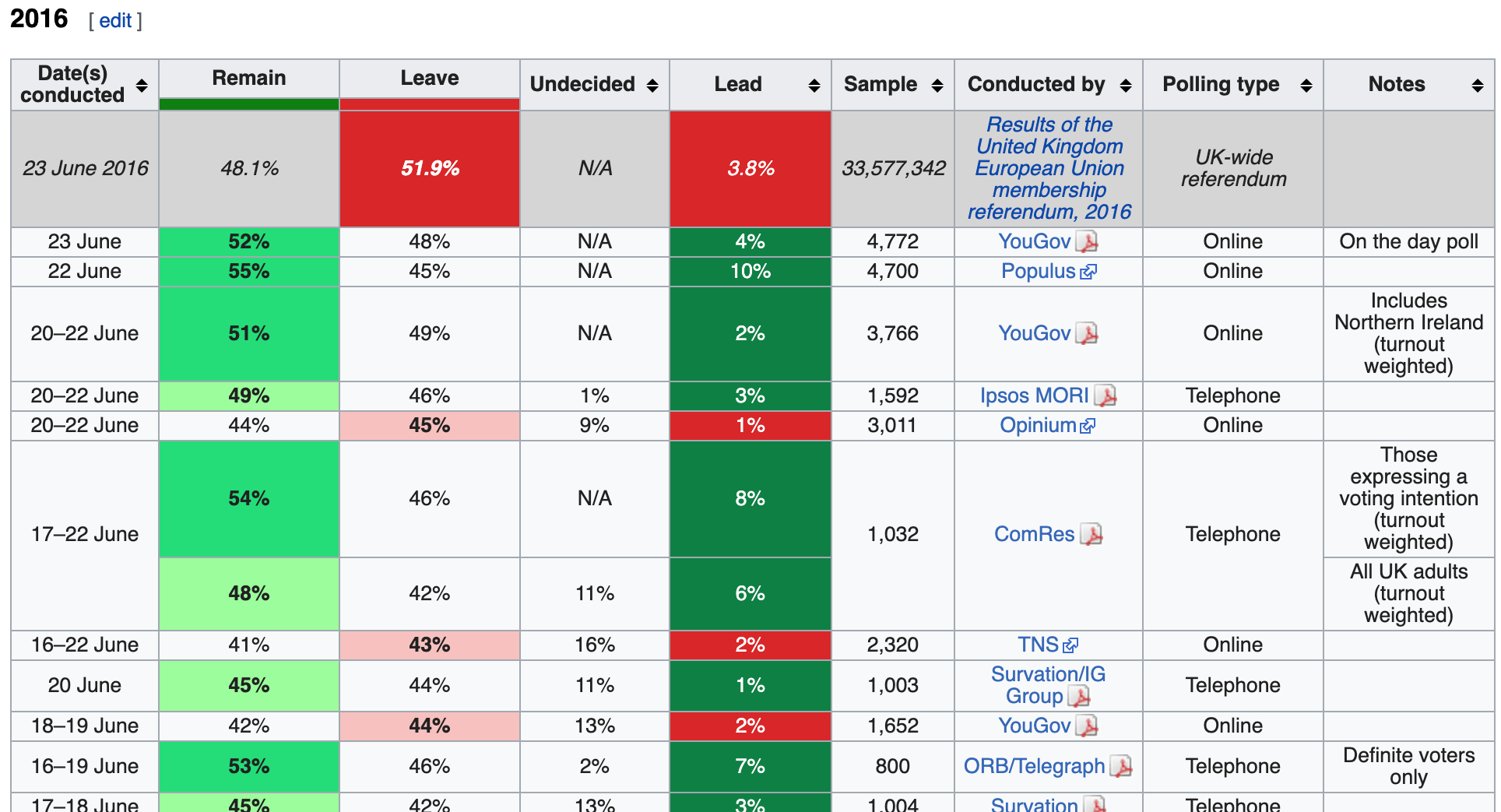
Polls regarding the referendum over 2016
Use the rvest library to read the HTML from this Wikipedia page (make sure to copy both lines of the URL):
url <- "https://en.wikipedia.org/w/index.php?title=Opinion_polling_for_the_United_Kingdom_European_Union_membership_referendum&oldid=896735054"Assign tab to be the html nodes of the “table” class.
How many tables are in this Wikipedia page?
tab <- read_html(url) %>% html_nodes("table")
length(tab)
## [1] 39- Inspect the first several html tables using
html_table()with the argumentfill=TRUE(you can read about this argument in the documentation). Find the first table that has 9 columns with the first column named “Date(s) conducted”.
What is the first table number to have 9 columns where the first column is named “Date(s) conducted”?
tab[[5]] %>% html_table(fill = TRUE) %>% names() # inspect column names## [1] "Date(s) conducted" "Remain" "Leave" "Undecided" "Lead" "Sample" "Conducted by" "Polling type"
## [9] "Notes"