3 Section 2 - Linear Models Overview

In the Linear Models section, you will learn how to do linear regression.

After completing this section, you will be able to:

Use multivariate regression to adjust for confounders.
Write linear models to describe the relationship between two or more variables.
Calculate the least squares estimates for a regression model using the lm function.
Understand the differences between tibbles and data frames.
Use the do() function to bridge R functions and the tidyverse.
Use the tidy(), glance(), and augment() functions from the broom package.
Apply linear regression to measurement error models.

This section has four parts: Introduction to Linear Models, Least Squares Estimates, Tibbles, do, and broom, and Regression and Baseball.

3.1 Confounding: Are BBs More Predictive?

The textbook for this section is available here

Key points

Association is not causation!
Although it may appear that BB cause runs, it is actually the HR that cause most of these runs. We say that BB are confounded with HR.
Regression can help us account for confounding.

Code

# find regression line for predicting runs from BBs
bb_slope <- Teams %>% 
  filter(yearID %in% 1961:2001 ) %>% 
  mutate(BB_per_game = BB/G, R_per_game = R/G) %>% 
  lm(R_per_game ~ BB_per_game, data = .) %>% 
  .$coef %>%
  .[2]
bb_slope

## BB_per_game 
##   0.7353288

# compute regression line for predicting runs from singles
singles_slope <- Teams %>% 
  filter(yearID %in% 1961:2001 ) %>%
  mutate(Singles_per_game = (H-HR-X2B-X3B)/G, R_per_game = R/G) %>%
  lm(R_per_game ~ Singles_per_game, data = .) %>%
  .$coef  %>%
  .[2]
singles_slope

## Singles_per_game 
##        0.4494253

# calculate correlation between HR, BB and singles
Teams %>% 
  filter(yearID %in% 1961:2001 ) %>% 
  mutate(Singles = (H-HR-X2B-X3B)/G, BB = BB/G, HR = HR/G) %>%  
  summarize(cor(BB, HR), cor(Singles, HR), cor(BB,Singles))

##   cor(BB, HR) cor(Singles, HR) cor(BB, Singles)
## 1   0.4039313       -0.1737435      -0.05603822

3.2 Stratification and Multivariate Regression

The textbook for this section is available here

Key points

A first approach to check confounding is to keep HRs fixed at a certain value and then examine the relationship between BB and runs.
The slopes of BB after stratifying on HR are reduced, but they are not 0, which indicates that BB are helpful for producing runs, just not as much as previously thought.

Code

# stratify HR per game to nearest 10, filter out strata with few points
dat <- Teams %>% filter(yearID %in% 1961:2001) %>%
  mutate(HR_strata = round(HR/G, 1), 
         BB_per_game = BB / G,
         R_per_game = R / G) %>%
  filter(HR_strata >= 0.4 & HR_strata <=1.2)
  
# scatterplot for each HR stratum
dat %>% 
  ggplot(aes(BB_per_game, R_per_game)) +  
  geom_point(alpha = 0.5) +
  geom_smooth(method = "lm") +
  facet_wrap( ~ HR_strata)

## `geom_smooth()` using formula 'y ~ x'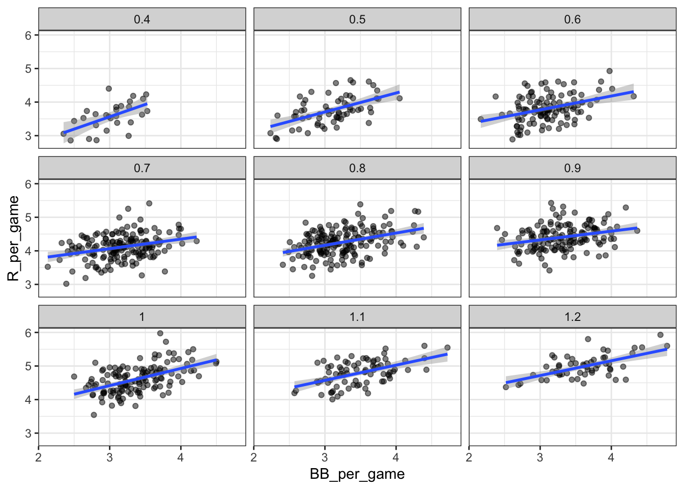

# calculate slope of regression line after stratifying by HR
dat %>%  
  group_by(HR_strata) %>%
  summarize(slope = cor(BB_per_game, R_per_game)*sd(R_per_game)/sd(BB_per_game))

## `summarise()` ungrouping output (override with `.groups` argument)

## # A tibble: 9 x 2
##   HR_strata slope
##       <dbl> <dbl>
## 1       0.4 0.734
## 2       0.5 0.566
## 3       0.6 0.412
## 4       0.7 0.285
## 5       0.8 0.365
## 6       0.9 0.261
## 7       1   0.512
## 8       1.1 0.454
## 9       1.2 0.440

# stratify by BB
dat <- Teams %>% filter(yearID %in% 1961:2001) %>%
  mutate(BB_strata = round(BB/G, 1), 
         HR_per_game = HR / G,
         R_per_game = R / G) %>%
  filter(BB_strata >= 2.8 & BB_strata <=3.9) 

# scatterplot for each BB stratum
dat %>% ggplot(aes(HR_per_game, R_per_game)) +  
  geom_point(alpha = 0.5) +
  geom_smooth(method = "lm") +
  facet_wrap( ~ BB_strata)

## `geom_smooth()` using formula 'y ~ x'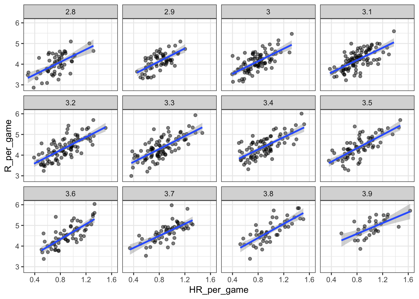

# slope of regression line after stratifying by BB
dat %>%  
  group_by(BB_strata) %>%
  summarize(slope = cor(HR_per_game, R_per_game)*sd(R_per_game)/sd(HR_per_game))

## `summarise()` ungrouping output (override with `.groups` argument)

## # A tibble: 12 x 2
##    BB_strata slope
##        <dbl> <dbl>
##  1       2.8  1.52
##  2       2.9  1.57
##  3       3    1.52
##  4       3.1  1.49
##  5       3.2  1.58
##  6       3.3  1.56
##  7       3.4  1.48
##  8       3.5  1.63
##  9       3.6  1.83
## 10       3.7  1.45
## 11       3.8  1.70
## 12       3.9  1.30

3.3 Linear Models

The textbook for this section is available here

Key points

“Linear” here does not refer to lines, but rather to the fact that the conditional expectation is a linear combination of known quantities.
In Galton’s model, we assume \(Y\) (son’s height) is a linear combination of a constant and \(X\) (father’s height) plus random noise. We further assume that \(\epsilon_i\) are independent from each other, have expected value 0 and the standard deviation \(\sigma\) which does not depend on i.
Note that if we further assume that \(\epsilon\) is normally distributed, then the model is exactly the same one we derived earlier by assuming bivariate normal data.
We can subtract the mean from \(X\) to make \(\beta_0\) more interpretable.

3.4 Assessment: Introduction to Linear Models

When we stratified our regression lines for runs per game vs. bases on balls by the number of home runs, what happened?

A. The slope of runs per game vs. bases on balls within each stratum was reduced because we removed confounding by home runs.
B. The slope of runs per game vs. bases on balls within each stratum was reduced because there were fewer data points.
C. The slope of runs per game vs. bases on balls within each stratum increased after we removed confounding by home runs.
D. The slope of runs per game vs. bases on balls within each stratum stayed about the same as the original slope.

We run a linear model for sons’ heights vs. fathers’ heights using the Galton height data, and get the following results:

> lm(son ~ father, data = galton_heights)

Call:
lm(formula = son ~ father, data = galton_heights)

Coefficients:
(Intercept)    father  
    35.71       0.50

Interpret the numeric coefficient for “father.”

A. For every inch we increase the son’s height, the predicted father’s height increases by 0.5 inches.
B. For every inch we increase the father’s height, the predicted son’s height grows by 0.5 inches.
C. For every inch we increase the father’s height, the predicted son’s height is 0.5 times greater.

We want the intercept term for our model to be more interpretable, so we run the same model as before but now we subtract the mean of fathers’ heights from each individual father’s height to create a new variable centered at zero.

galton_heights <- galton_heights %>%
    mutate(father_centered=father - mean(father))

We run a linear model using this centered fathers’ height variable.

> lm(son ~ father_centered, data = galton_heights)

Call:
lm(formula = son ~ father_centered, data = galton_heights)

Coefficients:
(Intercept)    father_centered  
    70.45          0.50

Interpret the numeric coefficient for the intercept.

A. The height of a son of a father of average height is 70.45 inches.
B. The height of a son when a father’s height is zero is 70.45 inches.
C. The height of an average father is 70.45 inches.

Suppose we fit a multivariate regression model for expected runs based on BB and HR:

\(E[R|BB=x_1, HR=x_2] = \beta_0+\beta_1x_1+\beta_2x_2\)

Suppose we fix \(BB = x_1\). Then we observe a linear relationship between runs and HR with intercept of:

A. \(\beta_0\)
B. \(\beta_0 + \beta_2x_2\)
C. \(\beta_0 + \beta_1x_1\)
D. \(\beta_0 + \beta_2x_1\)

Which of the following are assumptions for the errors \(\epsilon_i\) in a linear regression model? Check ALL correct answers.

A. The \(\epsilon_i\) are independent of each other
B. The \(\epsilon_i\) have expected value 0
C. The variance of \(\epsilon_i\) is a constant

3.5 Least Squares Estimates (LSE)

The textbook for this section is available here

Key points

For regression, we aim to find the coefficient values that minimize the distance of the fitted model to the data.
Residual sum of squares (RSS) measures the distance between the true value and the predicted value given by the regression line. The values that minimize the RSS are called the least squares estimates (LSE).
We can use partial derivatives to get the values for \(\beta_0\) and \(\beta_1\) in Galton’s data.

Code

# compute RSS for any pair of beta0 and beta1 in Galton's data
set.seed(1983)
galton_heights <- GaltonFamilies %>%
  filter(gender == "male") %>%
  group_by(family) %>%
  sample_n(1) %>%
  ungroup() %>%
  select(father, childHeight) %>%
  rename(son = childHeight)
rss <- function(beta0, beta1, data){
    resid <- galton_heights$son - (beta0+beta1*galton_heights$father)
    return(sum(resid^2))
}

# plot RSS as a function of beta1 when beta0=25
beta1 = seq(0, 1, len=nrow(galton_heights))
results <- data.frame(beta1 = beta1,
                      rss = sapply(beta1, rss, beta0 = 25))
results %>% ggplot(aes(beta1, rss)) + geom_line() + 
  geom_line(aes(beta1, rss))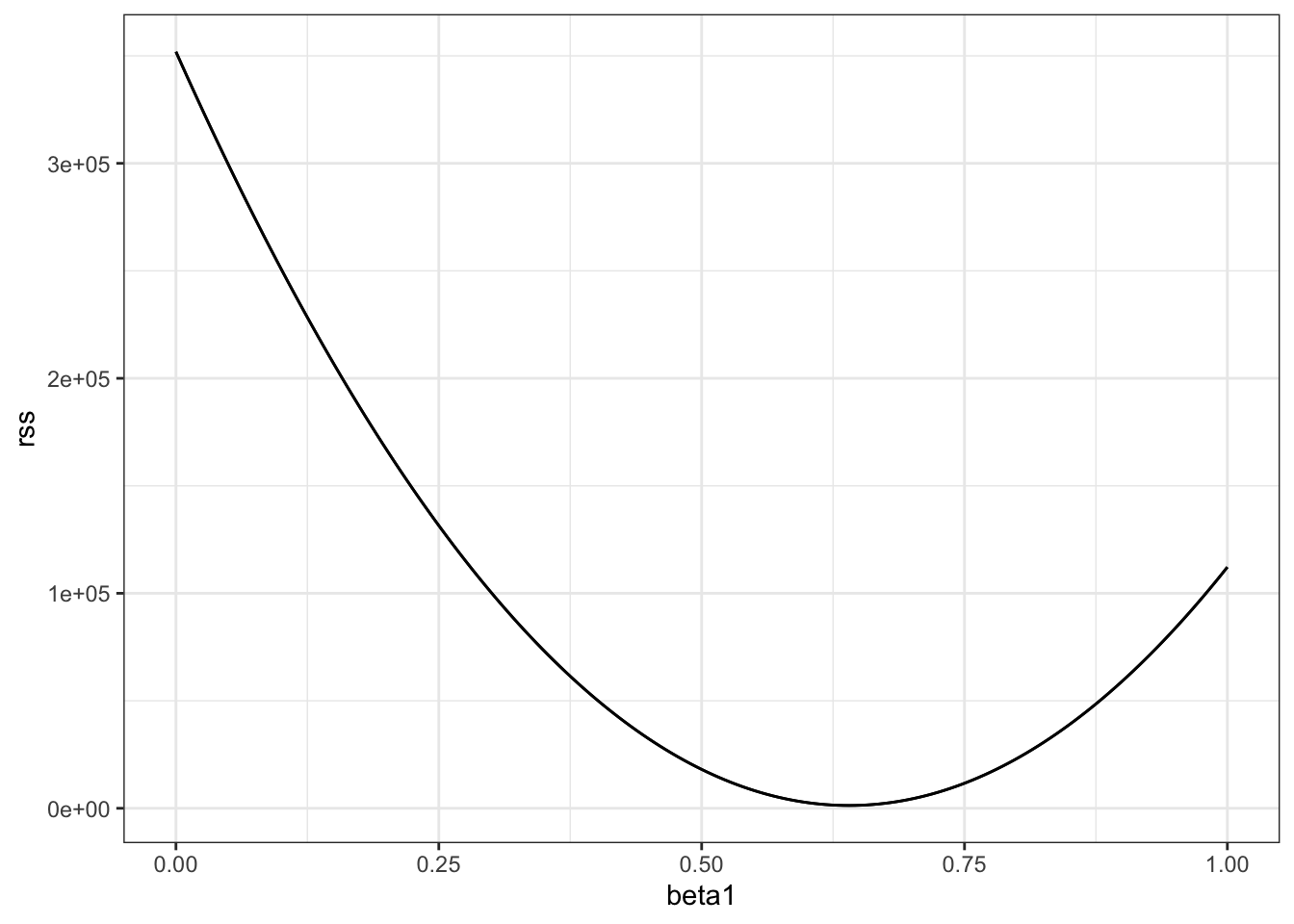

3.6 The lm Function

The textbook for this section is available here

Key points

When calling the lm() function, the variable that we want to predict is put to the left of the ~ symbol, and the variables that we use to predict is put to the right of the ~ symbol. The intercept is added automatically.
LSEs are random variables.

Code

# fit regression line to predict son's height from father's height
fit <- lm(son ~ father, data = galton_heights)
fit

## 
## Call:
## lm(formula = son ~ father, data = galton_heights)
## 
## Coefficients:
## (Intercept)       father  
##     38.7646       0.4411

# summary statistics
summary(fit)

## 
## Call:
## lm(formula = son ~ father, data = galton_heights)
## 
## Residuals:
##     Min      1Q  Median      3Q     Max 
## -9.4228 -1.7022  0.0333  1.5670  9.3567 
## 
## Coefficients:
##             Estimate Std. Error t value Pr(>|t|)    
## (Intercept) 38.76457    5.41093   7.164 2.03e-11 ***
## father       0.44112    0.07825   5.637 6.72e-08 ***
## ---
## Signif. codes:  0 '***' 0.001 '**' 0.01 '*' 0.05 '.' 0.1 ' ' 1
## 
## Residual standard error: 2.659 on 177 degrees of freedom
## Multiple R-squared:  0.1522, Adjusted R-squared:  0.1474 
## F-statistic: 31.78 on 1 and 177 DF,  p-value: 6.719e-08

3.7 LSE are Random Variables

The textbook for this section is available here

Key points

Because they are derived from the samples, LSE are random variables.
\(\beta_0\) and \(\beta_1\) appear to be normally distributed because the central limit theorem plays a role.
The t-statistic depends on the assumption that \(\epsilon\) follows a normal distribution.

Code

# Monte Carlo simulation
B <- 1000
N <- 50
lse <- replicate(B, {
  sample_n(galton_heights, N, replace = TRUE) %>% 
    lm(son ~ father, data = .) %>% 
    .$coef 
})
lse <- data.frame(beta_0 = lse[1,], beta_1 = lse[2,]) 

# Plot the distribution of beta_0 and beta_1
if(!require(gridExtra)) install.packages("gridExtra")

## Loading required package: gridExtra

## 
## Attaching package: 'gridExtra'

## The following object is masked from 'package:dplyr':
## 
##     combine

library(gridExtra)
p1 <- lse %>% ggplot(aes(beta_0)) + geom_histogram(binwidth = 5, color = "black") 
p2 <- lse %>% ggplot(aes(beta_1)) + geom_histogram(binwidth = 0.1, color = "black") 
grid.arrange(p1, p2, ncol = 2)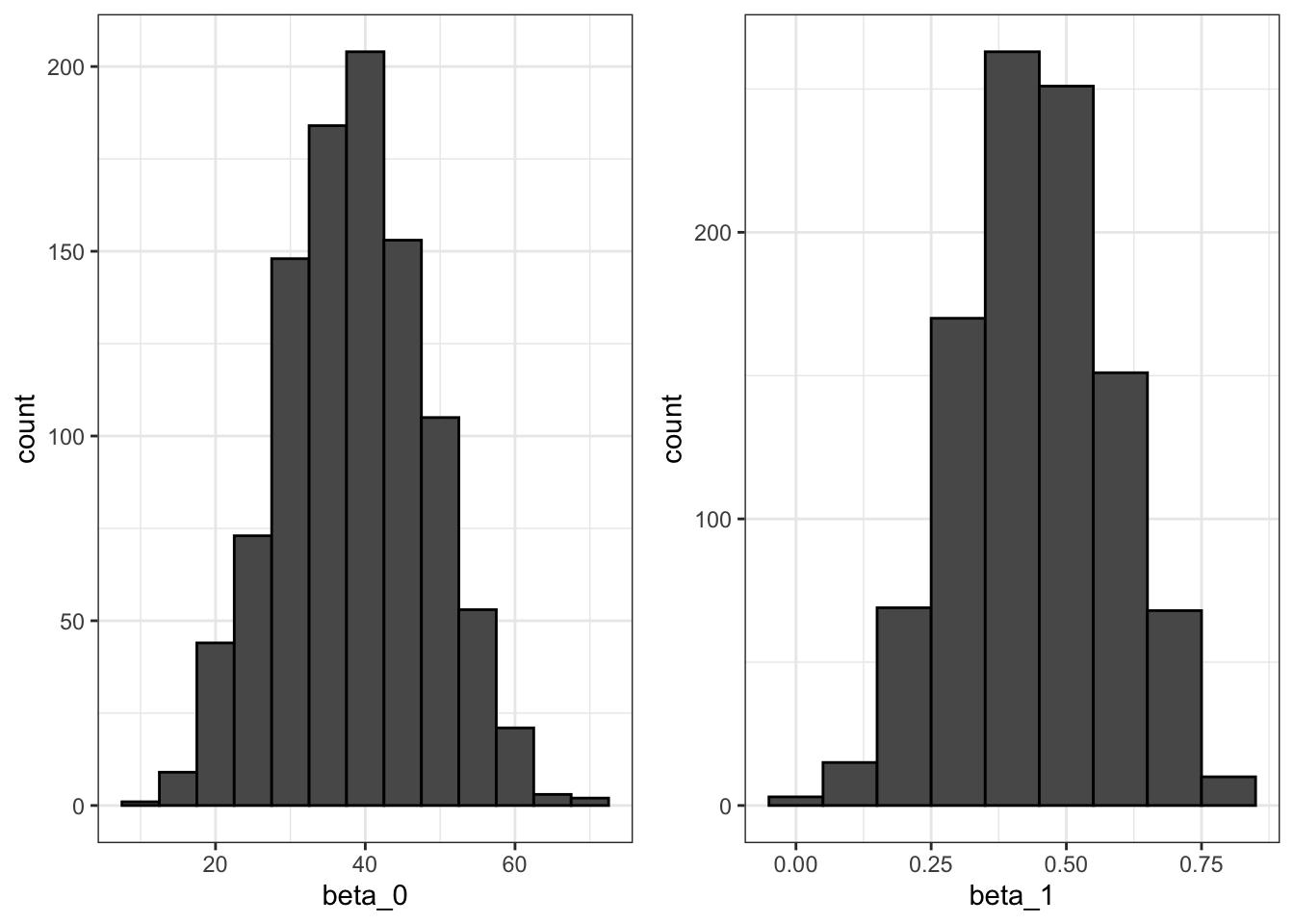

# summary statistics
sample_n(galton_heights, N, replace = TRUE) %>% 
  lm(son ~ father, data = .) %>% 
  summary %>%
  .$coef

##               Estimate Std. Error  t value     Pr(>|t|)
## (Intercept) 34.4729422  8.6021831 4.007464 0.0002129225
## father       0.4990193  0.1240572 4.022493 0.0002030210

lse %>% summarize(se_0 = sd(beta_0), se_1 = sd(beta_1))

##       se_0      se_1
## 1 9.683973 0.1411404

3.8 Advanced Note on LSE

Although interpretation is not straight-forward, it is also useful to know that the LSE can be strongly correlated, which can be seen using this code:

lse %>% summarize(cor(beta_0, beta_1))

##   cor(beta_0, beta_1)
## 1          -0.9993386

However, the correlation depends on how the predictors are defined or transformed.

Here we standardize the father heights, which changes \(x_i\) to \(x_i - \bar{x}\).

B <- 1000
N <- 50
lse <- replicate(B, {
      sample_n(galton_heights, N, replace = TRUE) %>%
      mutate(father = father - mean(father)) %>%
      lm(son ~ father, data = .) %>% .$coef 
})

Observe what happens to the correlation in this case:

cor(lse[1,], lse[2,])

## [1] 0.1100929

3.9 Predicted Variables are Random Variables

The textbook for this section is available here

Key points

The predicted value is often denoted as \(\hat{Y}\), which is a random variable. Mathematical theory tells us what the standard error of the predicted value is.
The predict() function in R can give us predictions directly.

Code

# plot predictions and confidence intervals
galton_heights %>% ggplot(aes(son, father)) +
  geom_point() +
  geom_smooth(method = "lm")

## `geom_smooth()` using formula 'y ~ x'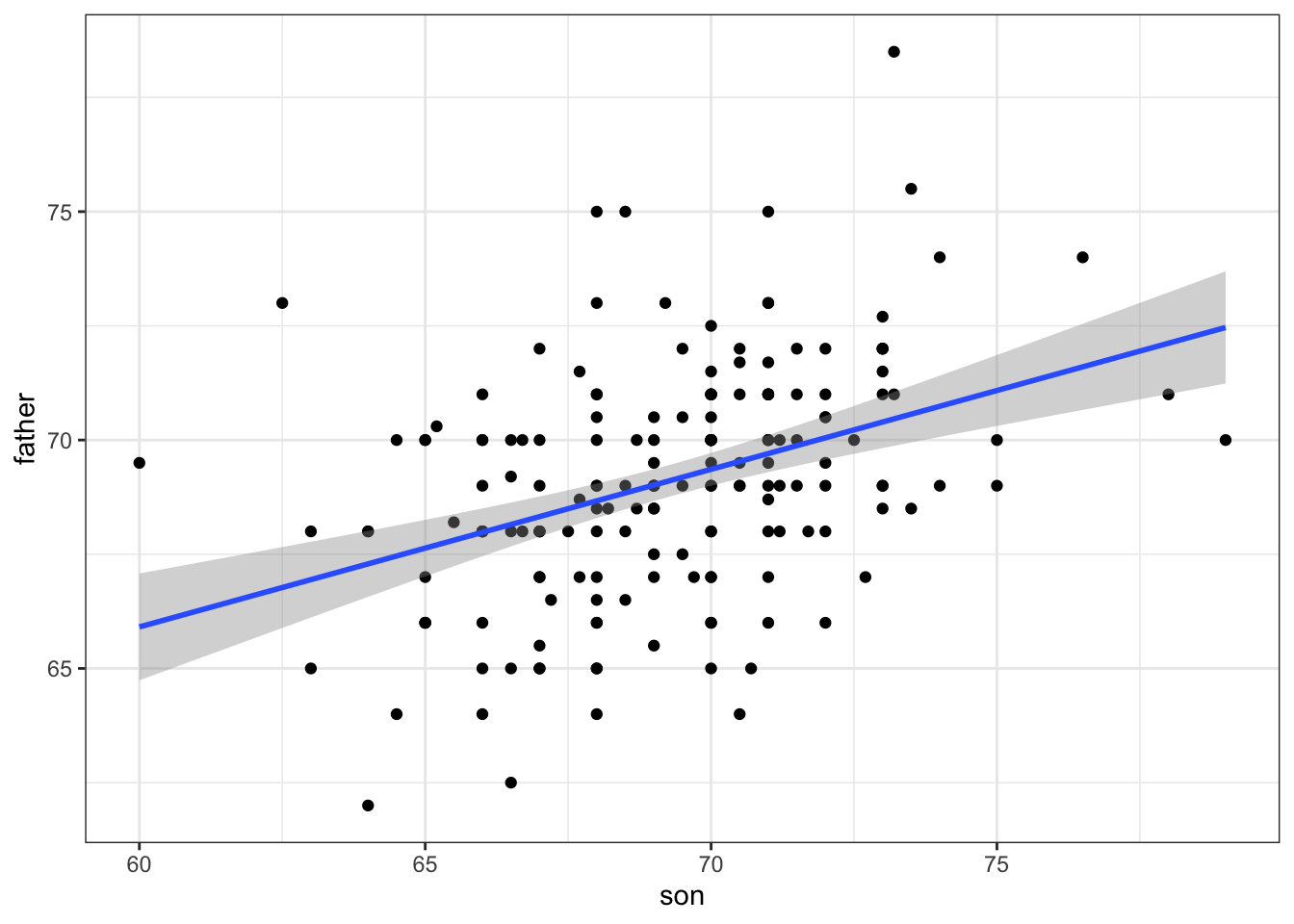

# predict Y directly
fit <- galton_heights %>% lm(son ~ father, data = .) 
Y_hat <- predict(fit, se.fit = TRUE)
names(Y_hat)

## [1] "fit"            "se.fit"         "df"             "residual.scale"

# plot best fit line
galton_heights %>%
  mutate(Y_hat = predict(lm(son ~ father, data=.))) %>%
  ggplot(aes(father, Y_hat))+
  geom_line()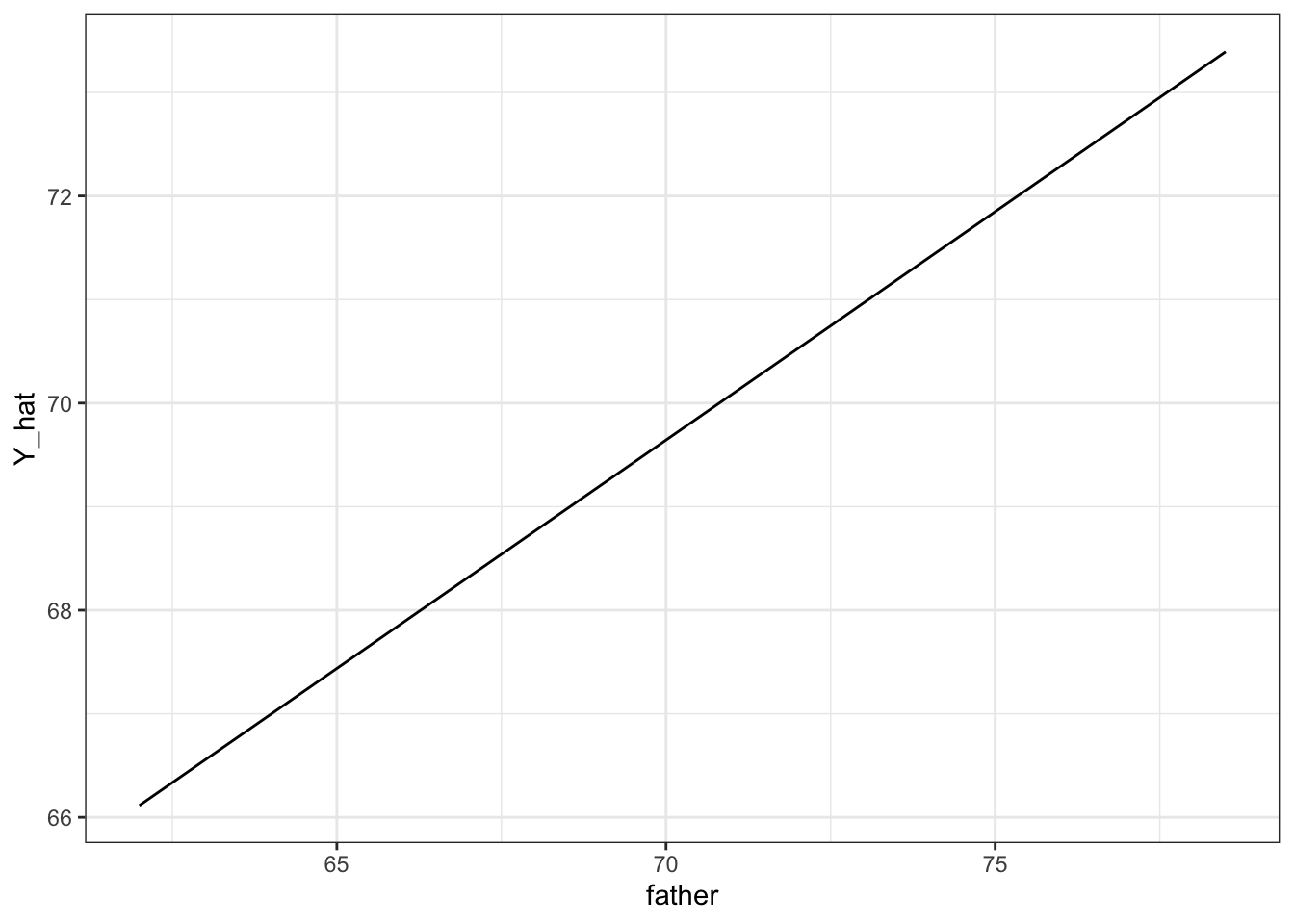

3.10 Assessment - Least Squares Estimates (LSE), part 1

The following code was used in the video to plot RSS with \(\beta_0=25\).

beta1 = seq(0, 1, len=nrow(galton_heights))
results <- data.frame(beta1 = beta1,
                      rss = sapply(beta1, rss, beta0 = 25))
results %>% ggplot(aes(beta1, rss)) + geom_line() + 
  geom_line(aes(beta1, rss), col=2)

In a model for sons’ heights vs fathers’ heights, what is the least squares estimate (LSE) for \(\beta_1\) if we assume \(\hat{\beta}_{0}\) is 36? Hint: modify the code above to do your analysis.

# compute RSS for any pair of beta0 and beta1 in Galton's data
set.seed(1983)
galton_heights <- GaltonFamilies %>%
  filter(gender == "male") %>%
  group_by(family) %>%
  sample_n(1) %>%
  ungroup() %>%
  select(father, childHeight) %>%
  rename(son = childHeight)
rss <- function(beta0, beta1, data){
    resid <- galton_heights$son - (beta0+beta1*galton_heights$father)
    return(sum(resid^2))
}

# plot RSS as a function of beta1 when beta0=36
beta1 = seq(0, 1, len=nrow(galton_heights))
results <- data.frame(beta1 = beta1,
                      rss = sapply(beta1, rss, beta0 = 36))
results %>% ggplot(aes(beta1, rss)) + geom_line() + 
  geom_line(aes(beta1, rss))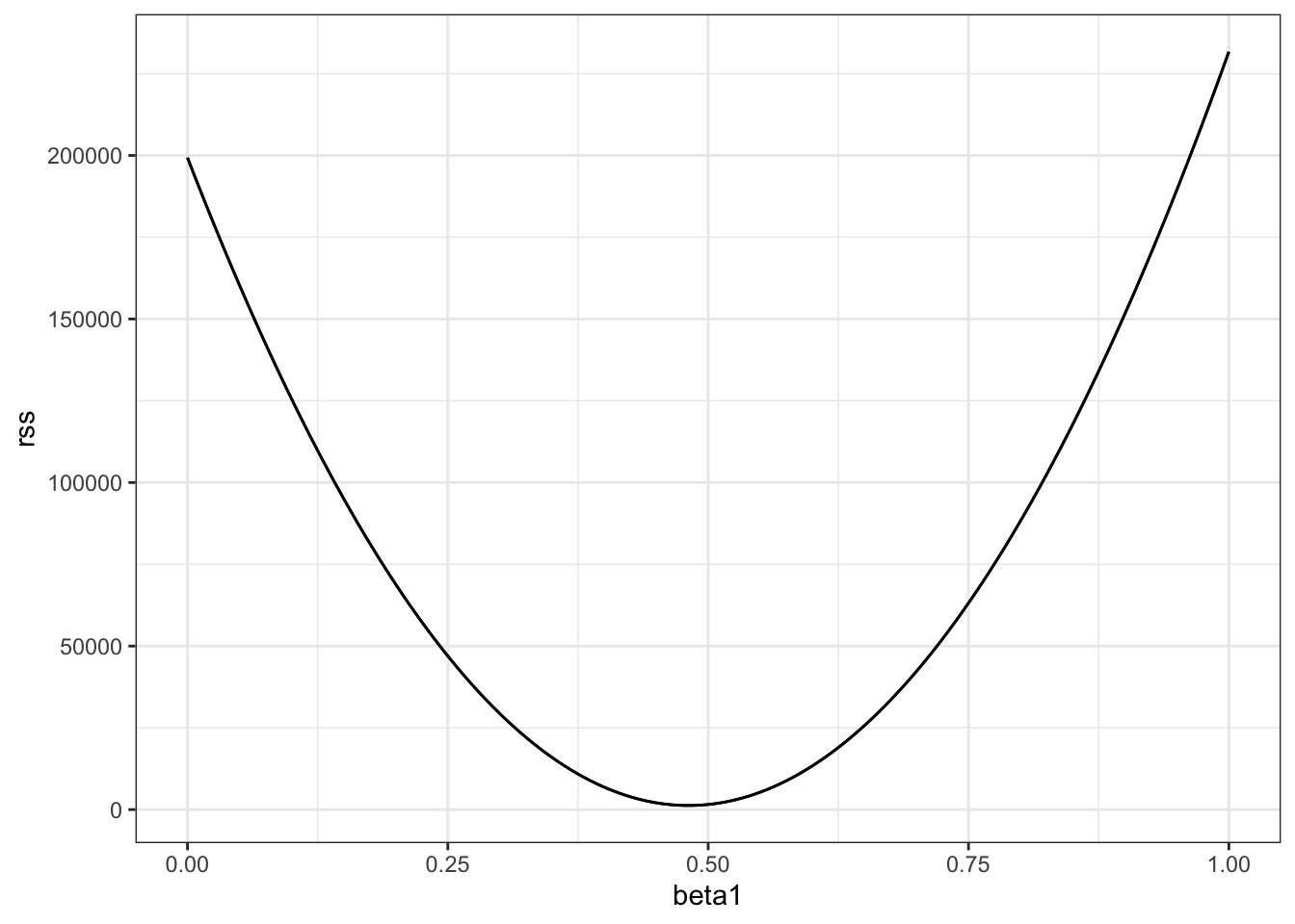

A. 0.65
B. 0.5
C. 0.2
D. 12

The least squares estimates for the parameters \(\beta_0, \beta_1, \dots, \beta_n\) minimize the residual sum of squares.
Load the Lahman library and filter the Teams data frame to the years 1961-2001.

Run a linear model in R predicting the number of runs per game based on the number of bases on balls and the number of home runs. Remember to first limit your data to 1961-2001.

What is the coefficient for bases on balls?

fit <- Teams %>% filter(yearID %in% 1961:2001) %>% 
mutate(R_per_game = R / G, BB_per_game = BB / G, HR_per_game = HR / G) %>% 
lm(R_per_game ~ BB_per_game + HR_per_game, data = .)

summary(fit)

## 
## Call:
## lm(formula = R_per_game ~ BB_per_game + HR_per_game, data = .)
## 
## Residuals:
##      Min       1Q   Median       3Q      Max 
## -0.87325 -0.24507 -0.01449  0.23866  1.24218 
## 
## Coefficients:
##             Estimate Std. Error t value Pr(>|t|)    
## (Intercept)  1.74430    0.08236   21.18   <2e-16 ***
## BB_per_game  0.38742    0.02701   14.34   <2e-16 ***
## HR_per_game  1.56117    0.04896   31.89   <2e-16 ***
## ---
## Signif. codes:  0 '***' 0.001 '**' 0.01 '*' 0.05 '.' 0.1 ' ' 1
## 
## Residual standard error: 0.3484 on 1023 degrees of freedom
## Multiple R-squared:  0.6503, Adjusted R-squared:  0.6496 
## F-statistic: 951.2 on 2 and 1023 DF,  p-value: < 2.2e-16

A. 0.39
B. 1.56
C. 1.74
D. 0.027

The coefficient for bases on balls is 0.39; the coefficient for home runs is 1.56; the intercept is 1.74; the standard error for the BB coefficient is 0.027.

We run a Monte Carlo simulation where we repeatedly take samples of N = 100 from the Galton heights data and compute the regression slope coefficients for each sample:

B <- 1000
N <- 100
lse <- replicate(B, {
    sample_n(galton_heights, N, replace = TRUE) %>% 
    lm(son ~ father, data = .) %>% .$coef 
})

lse <- data.frame(beta_0 = lse[1,], beta_1 = lse[2,])

What does the central limit theorem tell us about the variables beta_0 and beta_1?

A. They are approximately normally distributed.
B. The expected value of each is the true value of \(\beta_0\) and \(\beta_1\) (assuming the Galton heights data is a complete population).
C. The central limit theorem does not apply in this situation.
D. It allows us to test the hypothesis that \(\beta_0 = 0\) and \(\beta_0 = 1\)

In an earlier video, we ran the following linear model and looked at a summary of the results.

$\beta_0$
> mod <- lm(son ~ father, data = galton_heights)
> summary(mod)

Call:
lm(formula = son ~ father, data = galton_heights)

Residuals:
   Min     1Q  Median     3Q    Max 
-5.902  -1.405  0.092    1.342  8.092 

Coefficients:
                 Estimate  Std. Error  t value     Pr(>|t|)  
(Intercept)     35.7125     4.5174       7.91    2.8e-13 ***
father           0.5028     0.0653       7.70    9.5e-13 ***
---
Signif. codes:  0 ‘***’ 0.001 ‘**’ 0.01 ‘*’ 0.05 ‘.’ 0.1 ‘ ’ 1
$\beta_0$

What null hypothesis is the second p-value (the one in the father row) testing?

A. \(\beta_1 = 1\), where \(\beta_1\) is the coefficient for the variable “father.”
B. \(\beta_1 = 0.503\), where \(\beta_1\) is the coefficient for the variable “father.”
C. \(\beta_1 = 0\), where \(\beta_1\) is the coefficient for the variable “father.”

Which R code(s) below would properly plot the predictions and confidence intervals for our linear model of sons’ heights?

Select ALL that apply.

          galton_heights %>% ggplot(aes(father, son)) +
    geom_point() +
    geom_smooth()

          galton_heights %>% ggplot(aes(father, son)) +
    geom_point() +
    geom_smooth(method = "lm")

          model <- lm(son ~ father, data = galton_heights)
predictions <- predict(model, interval = c("confidence"), level = 0.95)
data <- as.tibble(predictions) %>% bind_cols(father = galton_heights$father)

ggplot(data, aes(x = father, y = fit)) +
    geom_line(color = "blue", size = 1) + 
    geom_ribbon(aes(ymin=lwr, ymax=upr), alpha=0.2) + 
    geom_point(data = galton_heights, aes(x = father, y = son))

          model <- lm(son ~ father, data = galton_heights)
predictions <- predict(model)
data <- as.tibble(predictions) %>% bind_cols(father = galton_heights$father)

ggplot(data, aes(x = father, y = fit)) +
    geom_line(color = "blue", size = 1) + 
    geom_point(data = galton_heights, aes(x = father, y = son))

3.11 Assessment - Least Squares Estimates, part 2

In Questions 7 and 8, you’ll look again at female heights from GaltonFamilies.

Define female_heights, a set of mother and daughter heights sampled from GaltonFamilies, as follows:

set.seed(1989, sample.kind="Rounding") #if you are using R 3.6 or later

## Warning in set.seed(1989, sample.kind = "Rounding"): non-uniform 'Rounding' sampler used

options(digits = 3)    # report 3 significant digits

female_heights <- GaltonFamilies %>%     
    filter(gender == "female") %>%     
    group_by(family) %>%     
    sample_n(1) %>%     
    ungroup() %>%     
    select(mother, childHeight) %>%     
    rename(daughter = childHeight)

Fit a linear regression model predicting the mothers’ heights using daughters’ heights.

What is the slope of the model?

fit <- lm(mother ~ daughter, data = female_heights)
fit$coef[2]

## daughter 
##     0.31

What the intercept of the model?

fit$coef[1]

## (Intercept) 
##        44.2

Predict mothers’ heights using the model.

What is the predicted height of the first mother in the dataset?

predict(fit)[1]

##    1 
## 65.6

What is the actual height of the first mother in the dataset?

female_heights$mother[1]

## [1] 67

We have shown how BB and singles have similar predictive power for scoring runs. Another way to compare the usefulness of these baseball metrics is by assessing how stable they are across the years. Because we have to pick players based on their previous performances, we will prefer metrics that are more stable. In these exercises, we will compare the stability of singles and BBs.

Before we get started, we want to generate two tables: one for 2002 and another for the average of 1999-2001 seasons. We want to define per plate appearance statistics, keeping only players with more than 100 plate appearances. Here is how we create the 2002 table:

bat_02 <- Batting %>% filter(yearID == 2002) %>%
    mutate(pa = AB + BB, singles = (H - X2B - X3B - HR)/pa, bb = BB/pa) %>%
    filter(pa >= 100) %>%
    select(playerID, singles, bb)

Now compute a similar table but with rates computed over 1999-2001. Keep only rows from 1999-2001 where players have 100 or more plate appearances, calculate each player’s single rate and BB rate per season, then calculate the average single rate (mean_singles) and average BB rate (mean_bb) per player over those three seasons.

How many players had a single rate mean_singles of greater than 0.2 per plate appearance over 1999-2001?

bat_99_01 <- Batting %>% filter(yearID %in% 1999:2001) %>%
    mutate(pa = AB + BB, singles = (H - X2B - X3B - HR)/pa, bb = BB/pa) %>%
    filter(pa >= 100) %>%
    group_by(playerID) %>%
    summarize(mean_singles = mean(singles), mean_bb = mean(bb))

## `summarise()` ungrouping output (override with `.groups` argument)

sum(bat_99_01$mean_singles > 0.2)

## [1] 46

How many players had a BB rate mean_bb of greater than 0.2 per plate appearance over 1999-2001?

sum(bat_99_01$mean_bb > 0.2)

## [1] 3

Use inner_join() to combine the `bat_02 table with the table of 1999-2001 rate averages you created in the previous question.

What is the correlation between 2002 singles rates and 1999-2001 average singles rates?

dat <- inner_join(bat_02, bat_99_01)

## Joining, by = "playerID"

cor(dat$singles, dat$mean_singles)

## [1] 0.551

What is the correlation between 2002 BB rates and 1999-2001 average BB rates?

cor(dat$bb, dat$mean_bb)

## [1] 0.717

Make scatterplots of mean_singles versus singles and mean_bb versus bb.

Are either of these distributions bivariate normal?

dat %>%
    ggplot(aes(singles, mean_singles)) +
    geom_point()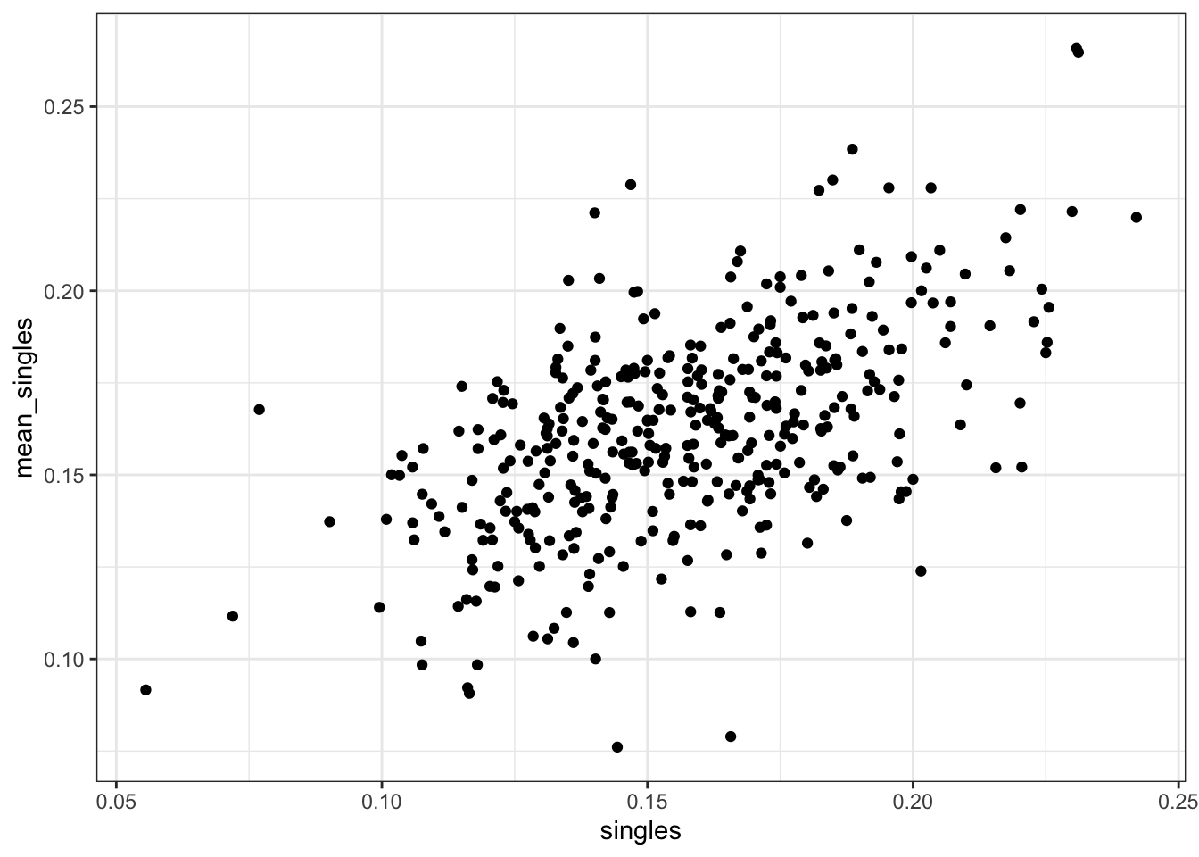

dat %>%
    ggplot(aes(bb, mean_bb)) +
    geom_point()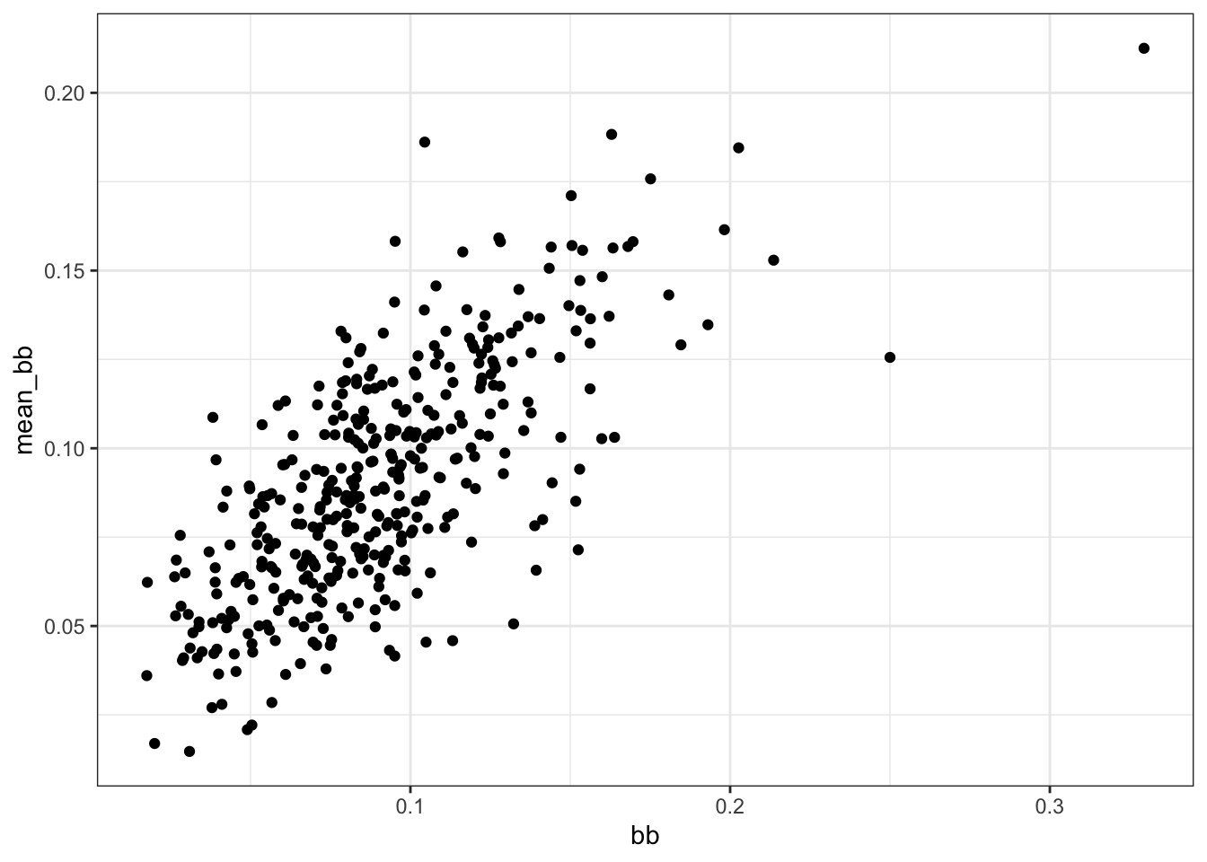

A. Neither distribution is bivariate normal.
B. singles and mean_singles are bivariate normal, but bb and mean_bb are not.
C. bb and mean_bb are bivariate normal, but singles and mean_singles are not.
D. Both distributions are bivariate normal.

Fit a linear model to predict 2002 singles given 1999-2001 mean_singles.

What is the coefficient of mean_singles, the slope of the fit?

fit_singles <- lm(singles ~ mean_singles, data = dat)
fit_singles$coef[2]

## mean_singles 
##        0.588

Fit a linear model to predict 2002 bb given 1999-2001 mean_bb.

What is the coefficient of mean_bb, the slope of the fit?

fit_bb <- lm(bb ~ mean_bb, data = dat)
fit_bb$coef[2]

## mean_bb 
##   0.829

3.12 Advanced dplyr: Tibbles

The textbook for this section is available here

Key points

Tibbles can be regarded as a modern version of data frames and are the default data structure in the tidyverse.
Some functions that do not work properly with data frames do work with tibbles.

Code

# stratify by HR
dat <- Teams %>% filter(yearID %in% 1961:2001) %>%
  mutate(HR = round(HR/G, 1), 
         BB = BB/G,
         R = R/G) %>%
  select(HR, BB, R) %>%
  filter(HR >= 0.4 & HR<=1.2)
  
# calculate slope of regression lines to predict runs by BB in different HR strata
dat %>%  
  group_by(HR) %>%
  summarize(slope = cor(BB,R)*sd(R)/sd(BB))

## `summarise()` ungrouping output (override with `.groups` argument)

## # A tibble: 9 x 2
##      HR slope
##   <dbl> <dbl>
## 1   0.4 0.734
## 2   0.5 0.566
## 3   0.6 0.412
## 4   0.7 0.285
## 5   0.8 0.365
## 6   0.9 0.261
## 7   1   0.512
## 8   1.1 0.454
## 9   1.2 0.440

# use lm to get estimated slopes - lm does not work with grouped tibbles
dat %>%  
  group_by(HR) %>%
  lm(R ~ BB, data = .) %>%
  .$coef

## (Intercept)          BB 
##       2.198       0.638

# inspect a grouped tibble
dat %>% group_by(HR) %>% head()

## # A tibble: 6 x 3
## # Groups:   HR [5]
##      HR    BB     R
##   <dbl> <dbl> <dbl>
## 1   0.9  3.56  4.24
## 2   0.7  3.97  4.47
## 3   0.8  3.37  4.69
## 4   1.1  3.46  4.42
## 5   1    2.75  4.61
## 6   0.9  3.06  4.58

dat %>% group_by(HR) %>% class()

## [1] "grouped_df" "tbl_df"     "tbl"        "data.frame"

3.13 Tibbles: Differences from Data Frames

Key points

Tibbles are more readable than data frames.
If you subset a data frame, you may not get a data frame. If you subset a tibble, you always get a tibble.
Tibbles can hold more complex objects such as lists or functions.
Tibbles can be grouped.

Code

# inspect data frame and tibble
head(Teams)

##   yearID lgID teamID franchID divID Rank  G Ghome  W  L DivWin WCWin LgWin WSWin   R   AB   H X2B X3B HR BB SO SB CS HBP SF  RA  ER  ERA CG SHO SV IPouts  HA HRA BBA SOA   E DP
## 1   1871   NA    BS1      BNA  <NA>    3 31    NA 20 10   <NA>  <NA>     N  <NA> 401 1372 426  70  37  3 60 19 73 16  NA NA 303 109 3.55 22   1  3    828 367   2  42  23 243 24
## 2   1871   NA    CH1      CNA  <NA>    2 28    NA 19  9   <NA>  <NA>     N  <NA> 302 1196 323  52  21 10 60 22 69 21  NA NA 241  77 2.76 25   0  1    753 308   6  28  22 229 16
## 3   1871   NA    CL1      CFC  <NA>    8 29    NA 10 19   <NA>  <NA>     N  <NA> 249 1186 328  35  40  7 26 25 18  8  NA NA 341 116 4.11 23   0  0    762 346  13  53  34 234 15
## 4   1871   NA    FW1      KEK  <NA>    7 19    NA  7 12   <NA>  <NA>     N  <NA> 137  746 178  19   8  2 33  9 16  4  NA NA 243  97 5.17 19   1  0    507 261   5  21  17 163  8
## 5   1871   NA    NY2      NNA  <NA>    5 33    NA 16 17   <NA>  <NA>     N  <NA> 302 1404 403  43  21  1 33 15 46 15  NA NA 313 121 3.72 32   1  0    879 373   7  42  22 235 14
## 6   1871   NA    PH1      PNA  <NA>    1 28    NA 21  7   <NA>  <NA>     Y  <NA> 376 1281 410  66  27  9 46 23 56 12  NA NA 266 137 4.95 27   0  0    747 329   3  53  16 194 13
##      FP                    name                         park attendance BPF PPF teamIDBR teamIDlahman45 teamIDretro
## 1 0.834    Boston Red Stockings          South End Grounds I         NA 103  98      BOS            BS1         BS1
## 2 0.829 Chicago White Stockings      Union Base-Ball Grounds         NA 104 102      CHI            CH1         CH1
## 3 0.818  Cleveland Forest Citys National Association Grounds         NA  96 100      CLE            CL1         CL1
## 4 0.803    Fort Wayne Kekiongas               Hamilton Field         NA 101 107      KEK            FW1         FW1
## 5 0.840        New York Mutuals     Union Grounds (Brooklyn)         NA  90  88      NYU            NY2         NY2
## 6 0.845  Philadelphia Athletics     Jefferson Street Grounds         NA 102  98      ATH            PH1         PH1

as_tibble(Teams)

## # A tibble: 2,925 x 48
##    yearID lgID  teamID franchID divID  Rank     G Ghome     W     L DivWin WCWin LgWin WSWin     R    AB     H   X2B   X3B    HR    BB    SO    SB    CS   HBP    SF    RA    ER   ERA
##     <int> <fct> <fct>  <fct>    <chr> <int> <int> <int> <int> <int> <chr>  <chr> <chr> <chr> <int> <int> <int> <int> <int> <int> <int> <int> <int> <int> <int> <int> <int> <int> <dbl>
##  1   1871 NA    BS1    BNA      <NA>      3    31    NA    20    10 <NA>   <NA>  N     <NA>    401  1372   426    70    37     3    60    19    73    16    NA    NA   303   109  3.55
##  2   1871 NA    CH1    CNA      <NA>      2    28    NA    19     9 <NA>   <NA>  N     <NA>    302  1196   323    52    21    10    60    22    69    21    NA    NA   241    77  2.76
##  3   1871 NA    CL1    CFC      <NA>      8    29    NA    10    19 <NA>   <NA>  N     <NA>    249  1186   328    35    40     7    26    25    18     8    NA    NA   341   116  4.11
##  4   1871 NA    FW1    KEK      <NA>      7    19    NA     7    12 <NA>   <NA>  N     <NA>    137   746   178    19     8     2    33     9    16     4    NA    NA   243    97  5.17
##  5   1871 NA    NY2    NNA      <NA>      5    33    NA    16    17 <NA>   <NA>  N     <NA>    302  1404   403    43    21     1    33    15    46    15    NA    NA   313   121  3.72
##  6   1871 NA    PH1    PNA      <NA>      1    28    NA    21     7 <NA>   <NA>  Y     <NA>    376  1281   410    66    27     9    46    23    56    12    NA    NA   266   137  4.95
##  7   1871 NA    RC1    ROK      <NA>      9    25    NA     4    21 <NA>   <NA>  N     <NA>    231  1036   274    44    25     3    38    30    53    10    NA    NA   287   108  4.3 
##  8   1871 NA    TRO    TRO      <NA>      6    29    NA    13    15 <NA>   <NA>  N     <NA>    351  1248   384    51    34     6    49    19    62    24    NA    NA   362   153  5.51
##  9   1871 NA    WS3    OLY      <NA>      4    32    NA    15    15 <NA>   <NA>  N     <NA>    310  1353   375    54    26     6    48    13    48    13    NA    NA   303   137  4.37
## 10   1872 NA    BL1    BLC      <NA>      2    58    NA    35    19 <NA>   <NA>  N     <NA>    617  2571   753   106    31    14    29    28    53    18    NA    NA   434   166  2.9 
## # … with 2,915 more rows, and 19 more variables: CG <int>, SHO <int>, SV <int>, IPouts <int>, HA <int>, HRA <int>, BBA <int>, SOA <int>, E <int>, DP <int>, FP <dbl>, name <chr>,
## #   park <chr>, attendance <int>, BPF <int>, PPF <int>, teamIDBR <chr>, teamIDlahman45 <chr>, teamIDretro <chr>

# Note that the function was formerly called as.tibble()

# subsetting a data frame sometimes generates vectors
class(Teams[,20])

## [1] "integer"

# subsetting a tibble always generates tibbles
class(as_tibble(Teams[,20]))

## [1] "tbl_df"     "tbl"        "data.frame"

# pulling a vector out of a tibble
class(as_tibble(Teams)$HR)

## [1] "integer"

# access a non-existing column in a data frame or a tibble
Teams$hr

## NULL

as_tibble(Teams)$HR

##    [1]   3  10   7   2   1   9   3   6   6  14   0   1   7   0   2   4   4   5   0   0   9   0   6  13   0   5   4   8   2   1   1  17   4   2   7   6   2   2  15   0   2   0   2   7
##   [45]   7   5   0   0   0   0   9   8   4   2   6   2   7   2   4   0   6   4   9   1   2   3   5   3   2   8   2  20   3   4   8  12   5   4   3  20   4   7   7   8   5   8  12   5
##   [89]  12   7  17  11   5   7  18   4  15  15  20   5  19   9   5  11  18  11  12  16   8   5  34  13   8  15  34  13  14  24   6  20   3  21  13   7   2  39  32  17  16  36  19 142
##  [133]  10  16  40  36  26  31  20   6  17   0  22  22  26  14   7  21   2   7  11  32   0   8   2   6   4  23  17  14  22  54  26  25  19  16  21  30  20   6   5  17   8   8  16  24
##  [177]  53  45  53  19  20  21  18  21  26  16  20  30  23  31  25  53  80  14  37  55  33  27  48  21  29  47  20  39  47  19  25  56  77  12  32  51  34  19  14  55  31  16  14  36
##  [221]  30  20  47  42  79  25  36  52  62  18  22  52  43  44  42  58  25  20   2  13  43  34  31  58  67  31  27  21  16  27  15  25  66  24  23  49  20  35  31  48  14  24  30  23
##  [265]  52  53  60  40  22  20  28  17  13  46  55  21  29  57  19  30  30  34  26  44  26  18  39  50  38  45  37  27  45  65  32  29  32  19  61  80  37  10  23  33  42 103  65  61
##  [309]  37  42  45  40  48  54  59  25  41  54  55  36  29  34  32  61  27  39  55  23  28  36  34  20  28  37  40  49  27  37  45  19  24  45  38  22  16  40  31  40  25  32  36  12
##  [353]  17  53  18  19  18  32  34  33  14  13  36  17  27  39  27  13  12  40  23  31  29  47  47  26  48  33  33  23  29  26  36  24  37  32  28  32  18  38  12  29  26  19  35  24
##  [397]  29  39  33  33  42  19  14  14   6  18  33  22   6  38   5  18  29  10  47  48  15  25  14   9  28  31  12  20  18  32  12  34  12   8  17  26  15  24  14  22  21  27  11  31
##  [441]  27  31  23  15  10  24  10  29  29  17  11  12  27  18  13  39  23  24  16  22  16  20  22  13  25  16   7  20  16  12  10  14  17  32  12  12  20   9  26  18  18  22   5  13
##  [485]  15  11  11  23  15  22  12  19  10  18  12  14  28  17   3  19  14  18  19  20  13  21  11  25  20  17   8  20  16  14   4  20  22  10  19  26  16  21  12  25  10  15   9  43
##  [529]  25  31   7  34  23   9  28  31  20  19  22  33  12  15   9  35  28  37  20  54  21  20  30  41  25  35  60  49  17  26  16  29  32  35  17  43  21  12  19  47  18  22  43  39
##  [573]  19  27  20  17  39  32  24  59  27  16  24  30   8  33  73  35  18  15  19  32  18  42  31  35  38  19  52  42  16  10  25  33  39  30  12  29  62  18  34  17  26  33  18  36
##  [617]  14  36  14  17  40  25  50  53  15  20  23  28  17  24  31  16  58  24  20  19  23  20  12  14  28  22  17  46  14  16  17  42  35  19  42  20  14  25  12  14  25  22  18  17
##  [661]  26  13  25  39  27  17  38   9  15  26   4  15  10  13   8  21  15   9  13  13  20  22  25  15   5  27   4  33  25  24  25  21  20  24  23  40  45  35  42  17  31  18  24  22
##  [705]  28  23  37  34  18  35  30  46 115  44  64  16  50  32  36  17  59  61  35  37  20  42  58  75 134  82  88  37  67  83  42  45  56  32  45  42  45  32  54  80  95 111 116  52
##  [749]  98 107  45  34  62  32  42  90  45  59  41  85 105  53 112  49  82  63  26  30  72  25  41  66  36  41  35  95  98  63  94  44  67  67  22  41  64  41  38  86  44  52  50 114
##  [793] 110  76 100  78 110 109  56  32  40  16  32  66  35  27  36  73 121  61  75  44  72  90  43  28  39  37  36  74  29  26  51 109 158  56  57  54  55  84  29  38  66  52  24  92
##  [837]  32  34  62 118 133  89  85  52  63 113  40  28  99  33  37 139  34  62 110 136 142 122 153  60  46 100  48  47 122  66  63 171  74  72  82 143 152 125 126  86  75 104  57  37
##  [881]  71  34  27  84  21  71  43 101 155 118  81  41  76  60  49  53 110  63  36  69  47  78  80 116 160 172 122  48  67  76  61  50  62  54  43  72  34  50  57  82 144 139  60  39
##  [925]  64  57  60  51  79  83  71 101  55 100  74 126 135 144  56  52  62 104  51  69  59  75  74  88  73  93 106 123 104 112  92  66  73  86  32  86  33  67  60  76  82 123  94  97
##  [969] 182  72 103  60  79  88  62 100  37  63  67  96  73 103 150 111 174  94 103  47  71  94  47  98  61  54  67  65 110 113 137 125
##  [ reached getOption("max.print") -- omitted 1925 entries ]

# create a tibble with complex objects
tibble(id = c(1, 2, 3), func = c(mean, median, sd))

## # A tibble: 3 x 2
##      id func  
##   <dbl> <list>
## 1     1 <fn>  
## 2     2 <fn>  
## 3     3 <fn>

3.14 do

The textbook for this section is available here

Key points

The do() function serves as a bridge between R functions, such as lm(), and the tidyverse.
We have to specify a column when using the do() function, otherwise we will get an error.
If the data frame being returned has more than one row, the rows will be concatenated appropriately.

Code

# use do to fit a regression line to each HR stratum
dat %>%  
    group_by(HR) %>%
    do(fit = lm(R ~ BB, data = .))

## # A tibble: 9 x 2
## # Rowwise: 
##      HR fit   
##   <dbl> <list>
## 1   0.4 <lm>  
## 2   0.5 <lm>  
## 3   0.6 <lm>  
## 4   0.7 <lm>  
## 5   0.8 <lm>  
## 6   0.9 <lm>  
## 7   1   <lm>  
## 8   1.1 <lm>  
## 9   1.2 <lm>

# using do without a column name gives an error
dat %>%
    group_by(HR) %>%
    do(lm(R ~ BB, data = .))

# define a function to extract slope from lm
get_slope <- function(data){
  fit <- lm(R ~ BB, data = data)
  data.frame(slope = fit$coefficients[2], 
             se = summary(fit)$coefficient[2,2])
}

# return the desired data frame
dat %>%  
  group_by(HR) %>%
  do(get_slope(.))

## # A tibble: 9 x 3
## # Groups:   HR [9]
##      HR slope     se
##   <dbl> <dbl>  <dbl>
## 1   0.4 0.734 0.208 
## 2   0.5 0.566 0.110 
## 3   0.6 0.412 0.0974
## 4   0.7 0.285 0.0705
## 5   0.8 0.365 0.0653
## 6   0.9 0.261 0.0751
## 7   1   0.512 0.0751
## 8   1.1 0.454 0.0855
## 9   1.2 0.440 0.0801

# not the desired output: a column containing data frames
dat %>%  
  group_by(HR) %>%
  do(slope = get_slope(.))

## # A tibble: 9 x 2
## # Rowwise: 
##      HR slope           
##   <dbl> <list>          
## 1   0.4 <df[,2] [1 × 2]>
## 2   0.5 <df[,2] [1 × 2]>
## 3   0.6 <df[,2] [1 × 2]>
## 4   0.7 <df[,2] [1 × 2]>
## 5   0.8 <df[,2] [1 × 2]>
## 6   0.9 <df[,2] [1 × 2]>
## 7   1   <df[,2] [1 × 2]>
## 8   1.1 <df[,2] [1 × 2]>
## 9   1.2 <df[,2] [1 × 2]>

# data frames with multiple rows will be concatenated appropriately
get_lse <- function(data){
  fit <- lm(R ~ BB, data = data)
  data.frame(term = names(fit$coefficients),
    estimate = fit$coefficients, 
    se = summary(fit)$coefficient[,2])
}

dat %>%  
  group_by(HR) %>%
  do(get_lse(.))

## # A tibble: 18 x 4
## # Groups:   HR [9]
##       HR term        estimate     se
##    <dbl> <chr>          <dbl>  <dbl>
##  1   0.4 (Intercept)    1.36  0.631 
##  2   0.4 BB             0.734 0.208 
##  3   0.5 (Intercept)    2.01  0.344 
##  4   0.5 BB             0.566 0.110 
##  5   0.6 (Intercept)    2.53  0.305 
##  6   0.6 BB             0.412 0.0974
##  7   0.7 (Intercept)    3.21  0.225 
##  8   0.7 BB             0.285 0.0705
##  9   0.8 (Intercept)    3.07  0.213 
## 10   0.8 BB             0.365 0.0653
## 11   0.9 (Intercept)    3.54  0.251 
## 12   0.9 BB             0.261 0.0751
## 13   1   (Intercept)    2.88  0.256 
## 14   1   BB             0.512 0.0751
## 15   1.1 (Intercept)    3.21  0.300 
## 16   1.1 BB             0.454 0.0855
## 17   1.2 (Intercept)    3.40  0.291 
## 18   1.2 BB             0.440 0.0801

3.15 broom

The textbook for this section is available here

Key points

The broom package has three main functions, all of which extract information from the object returned by lm and return it in a tidyverse friendly data frame.
The tidy() function returns estimates and related information as a data frame.
The functions glance() and augment() relate to model specific and observation specific outcomes respectively.

Code

# use tidy to return lm estimates and related information as a data frame
if(!require(broom)) install.packages("broom")

library(broom)
fit <- lm(R ~ BB, data = dat)
tidy(fit)

## # A tibble: 2 x 5
##   term        estimate std.error statistic  p.value
##   <chr>          <dbl>     <dbl>     <dbl>    <dbl>
## 1 (Intercept)    2.20     0.113       19.4 1.12e-70
## 2 BB             0.638    0.0344      18.5 1.35e-65

# add confidence intervals with tidy
tidy(fit, conf.int = TRUE)

## # A tibble: 2 x 7
##   term        estimate std.error statistic  p.value conf.low conf.high
##   <chr>          <dbl>     <dbl>     <dbl>    <dbl>    <dbl>     <dbl>
## 1 (Intercept)    2.20     0.113       19.4 1.12e-70    1.98      2.42 
## 2 BB             0.638    0.0344      18.5 1.35e-65    0.570     0.705

# pipeline with lm, do, tidy
dat %>%  
  group_by(HR) %>%
  do(tidy(lm(R ~ BB, data = .), conf.int = TRUE)) %>%
  filter(term == "BB") %>%
  select(HR, estimate, conf.low, conf.high)

## # A tibble: 9 x 4
## # Groups:   HR [9]
##      HR estimate conf.low conf.high
##   <dbl>    <dbl>    <dbl>     <dbl>
## 1   0.4    0.734    0.308     1.16 
## 2   0.5    0.566    0.346     0.786
## 3   0.6    0.412    0.219     0.605
## 4   0.7    0.285    0.146     0.425
## 5   0.8    0.365    0.236     0.494
## 6   0.9    0.261    0.112     0.409
## 7   1      0.512    0.363     0.660
## 8   1.1    0.454    0.284     0.624
## 9   1.2    0.440    0.280     0.601

# make ggplots
dat %>%  
  group_by(HR) %>%
  do(tidy(lm(R ~ BB, data = .), conf.int = TRUE)) %>%
  filter(term == "BB") %>%
  select(HR, estimate, conf.low, conf.high) %>%
  ggplot(aes(HR, y = estimate, ymin = conf.low, ymax = conf.high)) +
  geom_errorbar() +
  geom_point()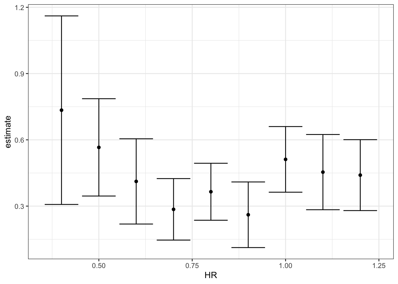

# inspect with glance
glance(fit)

## # A tibble: 1 x 12
##   r.squared adj.r.squared sigma statistic  p.value    df logLik   AIC   BIC deviance df.residual  nobs
##       <dbl>         <dbl> <dbl>     <dbl>    <dbl> <dbl>  <dbl> <dbl> <dbl>    <dbl>       <int> <int>
## 1     0.266         0.265 0.454      343. 1.35e-65     1  -596. 1199. 1214.     195.         947   949

3.16 Assessment - Tibbles, do, and broom, part 1

As seen in the videos, what problem do we encounter when we try to run a linear model on our baseball data, grouping by home runs?

A. There is not enough data in some levels to run the model.
B. The lm() function does not know how to handle grouped tibbles.
C. The results of the lm() function cannot be put into a tidy format.

Tibbles are similar to what other class in R?

A. Vectors
B. Matrices
C. Data frames
D. Lists

What are some advantages of tibbles compared to data frames?

A. Tibbles display better.
B. If you subset a tibble, you always get back a tibble.
C. Tibbles can have complex entries.
D. Tibbles can be grouped.

What are two advantages of the do command, when applied to the tidyverse?

A. It is faster than normal functions.
B. It returns useful error messages.
C. It understands grouped tibbles.
D. It always returns a data.frame.

You want to take the tibble dat, which we used in the video on the do() function, and run the linear model R ~ BB for each strata of HR. Then you want to add three new columns to your grouped tibble: the coefficient, standard error, and p-value for the BB term in the model.

You’ve already written the function get_slope(), shown below.

get_slope <- function(data) {
  fit <- lm(R ~ BB, data = data)
  sum.fit <- summary(fit)

  data.frame(slope = sum.fit$coefficients[2, "Estimate"], 
             se = sum.fit$coefficients[2, "Std. Error"],
             pvalue = sum.fit$coefficients[2, "Pr(>|t|)"])
}

What additional code could you write to accomplish your goal?

dat %>% 
  group_by(HR) %>% 
  do(get_slope(.))

## # A tibble: 9 x 4
## # Groups:   HR [9]
##      HR slope     se   pvalue
##   <dbl> <dbl>  <dbl>    <dbl>
## 1   0.4 0.734 0.208  1.54e- 3
## 2   0.5 0.566 0.110  3.02e- 6
## 3   0.6 0.412 0.0974 4.80e- 5
## 4   0.7 0.285 0.0705 7.93e- 5
## 5   0.8 0.365 0.0653 9.13e- 8
## 6   0.9 0.261 0.0751 6.85e- 4
## 7   1   0.512 0.0751 3.28e-10
## 8   1.1 0.454 0.0855 1.03e- 6
## 9   1.2 0.440 0.0801 1.07e- 6

dat %>% 
  group_by(HR) %>% 
  do(get_slope)

dat %>% 
  group_by(HR) %>% 
  do(get_slope(.))

dat %>% 
  group_by(HR) %>% 
  do(slope = get_slope(.))

dat %>% 
  do(get_slope(.))

The output of a broom function is always what?

A. A data.frame
B. A list
C. A vector

You want to know whether the relationship between home runs and runs per game varies by baseball league.

You create the following dataset:

dat <- Teams %>% filter(yearID %in% 1961:2001) %>%
  mutate(HR = HR/G,
         R = R/G) %>%
  select(lgID, HR, BB, R)

What code would help you quickly answer this question?

dat %>% 
  group_by(lgID) %>% 
  do(tidy(lm(R ~ HR, data = .), conf.int = T)) %>% 
  filter(term == "HR")

## # A tibble: 2 x 8
## # Groups:   lgID [2]
##   lgID  term  estimate std.error statistic  p.value conf.low conf.high
##   <fct> <chr>    <dbl>     <dbl>     <dbl>    <dbl>    <dbl>     <dbl>
## 1 AL    HR        1.90    0.0734      25.9 1.29e-95     1.75      2.04
## 2 NL    HR        1.76    0.0671      26.2 1.16e-95     1.62      1.89

dat %>% 
  group_by(lgID) %>% 
  do(tidy(lm(R ~ HR, data = .), conf.int = T)) %>% 
  filter(term == "HR")

dat %>% 
  group_by(lgID) %>% 
  do(glance(lm(R ~ HR, data = .)))

dat %>% 
  do(tidy(lm(R ~ HR, data = .), conf.int = T)) %>% 
  filter(term == "HR")

dat %>% 
  group_by(lgID) %>% 
  do(mod = lm(R ~ HR, data = .))

3.17 Assessment - Tibbles, do, and broom, part 2

We have investigated the relationship between fathers’ heights and sons’ heights. But what about other parent-child relationships? Does one parent’s height have a stronger association with child height? How does the child’s gender affect this relationship in heights? Are any differences that we observe statistically significant?

The galton dataset is a sample of one male and one female child from each family in the GaltonFamilies dataset. The pair column denotes whether the pair is father and daughter, father and son, mother and daughter, or mother and son.

Create the galton dataset using the code below:

data("GaltonFamilies")
set.seed(1) # if you are using R 3.5 or earlier
set.seed(1, sample.kind = "Rounding") # if you are using R 3.6 or later

## Warning in set.seed(1, sample.kind = "Rounding"): non-uniform 'Rounding' sampler used

galton <- GaltonFamilies %>%
    group_by(family, gender) %>%
    sample_n(1) %>%
    ungroup() %>% 
    gather(parent, parentHeight, father:mother) %>%
    mutate(child = ifelse(gender == "female", "daughter", "son")) %>%
    unite(pair, c("parent", "child"))

galton

## # A tibble: 710 x 8
##    family midparentHeight children childNum gender childHeight pair            parentHeight
##    <fct>            <dbl>    <int>    <int> <fct>        <dbl> <chr>                  <dbl>
##  1 001               75.4        4        2 female        69.2 father_daughter         78.5
##  2 001               75.4        4        1 male          73.2 father_son              78.5
##  3 002               73.7        4        4 female        65.5 father_daughter         75.5
##  4 002               73.7        4        2 male          72.5 father_son              75.5
##  5 003               72.1        2        2 female        68   father_daughter         75  
##  6 003               72.1        2        1 male          71   father_son              75  
##  7 004               72.1        5        5 female        63   father_daughter         75  
##  8 004               72.1        5        2 male          68.5 father_son              75  
##  9 005               69.1        6        5 female        62.5 father_daughter         75  
## 10 005               69.1        6        1 male          72   father_son              75  
## # … with 700 more rows

Group by pair and summarize the number of observations in each group.

How many father-daughter pairs are in the dataset?

How many mother-son pairs are in the dataset?

galton %>%
    group_by(pair) %>%
    summarize(n = n())

## `summarise()` ungrouping output (override with `.groups` argument)

## # A tibble: 4 x 2
##   pair                n
##   <chr>           <int>
## 1 father_daughter   176
## 2 father_son        179
## 3 mother_daughter   176
## 4 mother_son        179

Calculate the correlation coefficients for fathers and daughters, fathers and sons, mothers and daughters and mothers and sons.

Which pair has the strongest correlation in heights?

galton %>%
    group_by(pair) %>%
    summarize(cor = cor(parentHeight, childHeight)) %>%
    filter(cor == max(cor))

## `summarise()` ungrouping output (override with `.groups` argument)

## # A tibble: 1 x 2
##   pair         cor
##   <chr>      <dbl>
## 1 father_son 0.430

Which pair has the weakest correlation in heights?

galton %>%
    group_by(pair) %>%
    summarize(cor = cor(parentHeight, childHeight)) %>%
    filter(cor == min(cor))

## `summarise()` ungrouping output (override with `.groups` argument)

## # A tibble: 1 x 2
##   pair         cor
##   <chr>      <dbl>
## 1 mother_son 0.343

Question 10 has two parts. The information here applies to both parts.

Use lm() and the broom package to fit regression lines for each parent-child pair type. Compute the least squares estimates, standard errors, confidence intervals and p-values for the parentHeight coefficient for each pair.

10a. What is the estimate of the father-daughter coefficient?

galton %>%
    group_by(pair) %>%
    do(tidy(lm(childHeight ~ parentHeight, data = .), conf.int = TRUE)) %>%
    filter(term == "parentHeight", pair == "father_daughter") %>%
    pull(estimate)

## [1] 0.345

For every 1-inch increase in mother’s height, how many inches does the typical son’s height increase?

galton %>%
    group_by(pair) %>%
    do(tidy(lm(childHeight ~ parentHeight, data = .), conf.int = TRUE)) %>%
    filter(term == "parentHeight", pair == "mother_son") %>%
    pull(estimate)

## [1] 0.381

10b. Which sets of parent-child heights are significantly correlated at a p-value cut off of .05?

galton %>%
    group_by(pair) %>%
    do(tidy(lm(childHeight ~ parentHeight, data = .), conf.int = TRUE)) %>%
    filter(term == "parentHeight" & p.value < .05)

## # A tibble: 4 x 8
## # Groups:   pair [4]
##   pair            term         estimate std.error statistic       p.value conf.low conf.high
##   <chr>           <chr>           <dbl>     <dbl>     <dbl>         <dbl>    <dbl>     <dbl>
## 1 father_daughter parentHeight    0.345    0.0599      5.77 0.0000000356     0.227     0.464
## 2 father_son      parentHeight    0.443    0.0700      6.33 0.00000000194    0.305     0.581
## 3 mother_daughter parentHeight    0.394    0.0720      5.47 0.000000156      0.252     0.536
## 4 mother_son      parentHeight    0.381    0.0784      4.86 0.00000259       0.226     0.535

A. father-daughter
B. father-son
C. mother-daughter
D. mother-son

Which of the following statements are true?

A. All of the confidence intervals overlap each other.
B. At least one confidence interval covers zero.
C. The confidence intervals involving mothers’ heights are larger than the confidence intervals involving fathers’ heights.
D. The confidence intervals involving daughters’ heights are larger than the confidence intervals involving sons’ heights.
E. The data are consistent with inheritance of height being independent of the child’s gender.
F. The data are consistent with inheritance of height being independent of the parent’s gender.

3.18 Building a Better Offensive Metric for Baseball

The textbook for this section is available here

Code

# linear regression with two variables
fit <- Teams %>% 
  filter(yearID %in% 1961:2001) %>% 
  mutate(BB = BB/G, HR = HR/G,  R = R/G) %>%  
  lm(R ~ BB + HR, data = .)
  tidy(fit, conf.int = TRUE)

## # A tibble: 3 x 7
##   term        estimate std.error statistic   p.value conf.low conf.high
##   <chr>          <dbl>     <dbl>     <dbl>     <dbl>    <dbl>     <dbl>
## 1 (Intercept)    1.74     0.0824      21.2 7.62e- 83    1.58      1.91 
## 2 BB             0.387    0.0270      14.3 1.20e- 42    0.334     0.440
## 3 HR             1.56     0.0490      31.9 1.78e-155    1.47      1.66

# regression with BB, singles, doubles, triples, HR
fit <- Teams %>% 
  filter(yearID %in% 1961:2001) %>% 
  mutate(BB = BB / G, 
         singles = (H - X2B - X3B - HR) / G, 
         doubles = X2B / G, 
         triples = X3B / G, 
         HR = HR / G,
         R = R / G) %>%  
  lm(R ~ BB + singles + doubles + triples + HR, data = .)
coefs <- tidy(fit, conf.int = TRUE)
coefs

## # A tibble: 6 x 7
##   term        estimate std.error statistic   p.value conf.low conf.high
##   <chr>          <dbl>     <dbl>     <dbl>     <dbl>    <dbl>     <dbl>
## 1 (Intercept)   -2.77     0.0862     -32.1 4.76e-157   -2.94     -2.60 
## 2 BB             0.371    0.0117      31.6 1.87e-153    0.348     0.394
## 3 singles        0.519    0.0127      40.8 8.67e-217    0.494     0.544
## 4 doubles        0.771    0.0226      34.1 8.44e-171    0.727     0.816
## 5 triples        1.24     0.0768      16.1 2.12e- 52    1.09      1.39 
## 6 HR             1.44     0.0243      59.3 0.           1.40      1.49

# predict number of runs for each team in 2002 and plot
Teams %>% 
  filter(yearID %in% 2002) %>% 
  mutate(BB = BB/G, 
         singles = (H-X2B-X3B-HR)/G, 
         doubles = X2B/G, 
         triples =X3B/G, 
         HR=HR/G,
         R=R/G)  %>% 
  mutate(R_hat = predict(fit, newdata = .)) %>%
  ggplot(aes(R_hat, R, label = teamID)) + 
  geom_point() +
  geom_text(nudge_x=0.1, cex = 2) + 
  geom_abline()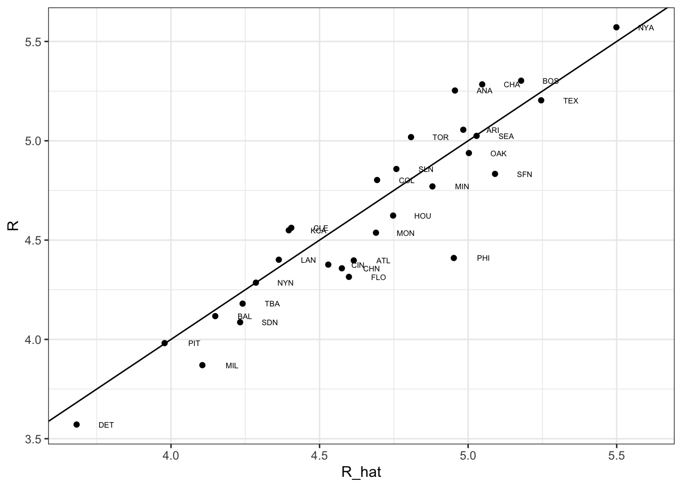

# average number of team plate appearances per game
pa_per_game <- Batting %>% filter(yearID == 2002) %>% 
  group_by(teamID) %>%
  summarize(pa_per_game = sum(AB+BB)/max(G)) %>% 
  pull(pa_per_game) %>% 
  mean

## `summarise()` ungrouping output (override with `.groups` argument)

# compute per-plate-appearance rates for players available in 2002 using previous data
players <- Batting %>% filter(yearID %in% 1999:2001) %>% 
  group_by(playerID) %>%
  mutate(PA = BB + AB) %>%
  summarize(G = sum(PA)/pa_per_game,
    BB = sum(BB)/G,
    singles = sum(H-X2B-X3B-HR)/G,
    doubles = sum(X2B)/G, 
    triples = sum(X3B)/G, 
    HR = sum(HR)/G,
    AVG = sum(H)/sum(AB),
    PA = sum(PA)) %>%
  filter(PA >= 300) %>%
  select(-G) %>%
  mutate(R_hat = predict(fit, newdata = .))

## `summarise()` ungrouping output (override with `.groups` argument)

# plot player-specific predicted runs
qplot(R_hat, data = players, geom = "histogram", binwidth = 0.5, color = I("black"))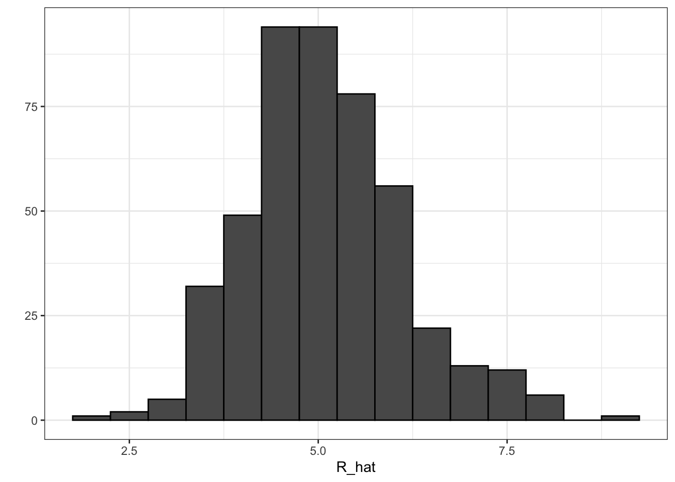

# add 2002 salary of each player
players <- Salaries %>% 
  filter(yearID == 2002) %>%
  select(playerID, salary) %>%
  right_join(players, by="playerID")
  
# add defensive position
position_names <- c("G_p","G_c","G_1b","G_2b","G_3b","G_ss","G_lf","G_cf","G_rf")
tmp_tab <- Appearances %>% 
  filter(yearID == 2002) %>% 
  group_by(playerID) %>%
  summarize_at(position_names, sum) %>%
  ungroup()  
pos <- tmp_tab %>%
  select(position_names) %>%
  apply(., 1, which.max)

## Note: Using an external vector in selections is ambiguous.
## ℹ Use `all_of(position_names)` instead of `position_names` to silence this message.
## ℹ See <https://tidyselect.r-lib.org/reference/faq-external-vector.html>.
## This message is displayed once per session.

players <- data_frame(playerID = tmp_tab$playerID, POS = position_names[pos]) %>%
  mutate(POS = str_to_upper(str_remove(POS, "G_"))) %>%
  filter(POS != "P") %>%
  right_join(players, by="playerID") %>%
  filter(!is.na(POS)  & !is.na(salary))

## Warning: `data_frame()` is deprecated as of tibble 1.1.0.
## Please use `tibble()` instead.
## This warning is displayed once every 8 hours.
## Call `lifecycle::last_warnings()` to see where this warning was generated.

# add players' first and last names
players <- Master %>%
  select(playerID, nameFirst, nameLast, debut) %>%
  mutate(debut = as.Date(debut)) %>%
  right_join(players, by="playerID")
  
# top 10 players
players %>% select(nameFirst, nameLast, POS, salary, R_hat) %>% 
  arrange(desc(R_hat)) %>% 
  top_n(10)

## Selecting by R_hat

##    nameFirst    nameLast POS   salary R_hat
## 1      Barry       Bonds  LF 15000000  9.05
## 2       Todd      Helton  1B  5000000  8.23
## 3      Manny     Ramirez  LF 15462727  8.20
## 4      Sammy        Sosa  RF 15000000  8.19
## 5      Larry      Walker  RF 12666667  8.15
## 6      Jason      Giambi  1B 10428571  7.99
## 7    Chipper       Jones  LF 11333333  7.64
## 8      Brian       Giles  LF  8063003  7.57
## 9     Albert      Pujols  LF   600000  7.54
## 10     Nomar Garciaparra  SS  9000000  7.51

# players with a higher metric have higher salaries
players %>% ggplot(aes(salary, R_hat, color = POS)) + 
  geom_point() +
  scale_x_log10()

# remake plot without players that debuted after 1998
if(!require(lubridate)) install.packages("lubridate")

## Loading required package: lubridate

## 
## Attaching package: 'lubridate'

## The following objects are masked from 'package:base':
## 
##     date, intersect, setdiff, union

library(lubridate)
players %>% filter(year(debut) < 1998) %>%
 ggplot(aes(salary, R_hat, color = POS)) + 
  geom_point() +
  scale_x_log10()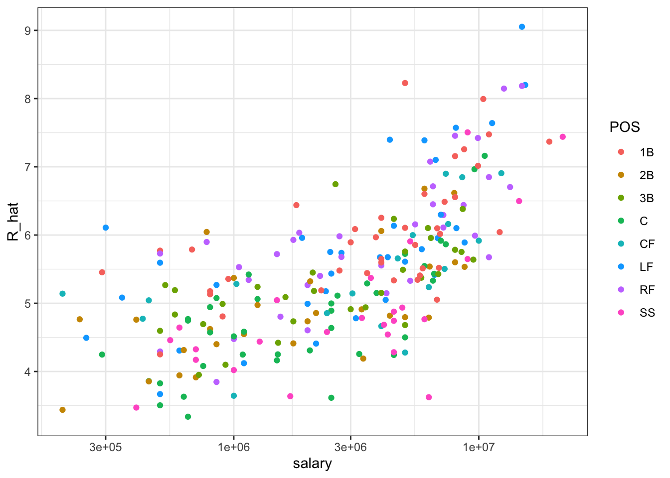

3.19 Building a Better Offensive Metric for Baseball: Linear Programming

A way to actually pick the players for the team can be done using what computer scientists call linear programming. Although we don’t go into this topic in detail in this course, we include the code anyway:

if(!require(reshape2)) install.packages("reshape2")

## Loading required package: reshape2

## 
## Attaching package: 'reshape2'

## The following object is masked from 'package:tidyr':
## 
##     smiths

if(!require(lpSolve)) install.packages("lpSolve")

## Loading required package: lpSolve

library(reshape2)
library(lpSolve)

players <- players %>% filter(debut <= "1997-01-01" & debut > "1988-01-01")
constraint_matrix <- acast(players, POS ~ playerID, fun.aggregate = length)

## Using R_hat as value column: use value.var to override.

npos <- nrow(constraint_matrix)
constraint_matrix <- rbind(constraint_matrix, salary = players$salary)
constraint_dir <- c(rep("==", npos), "<=")
constraint_limit <- c(rep(1, npos), 50*10^6)
lp_solution <- lp("max", players$R_hat,
                  constraint_matrix, constraint_dir, constraint_limit,
                  all.int = TRUE)

This algorithm chooses these 9 players:

our_team <- players %>%
  filter(lp_solution$solution == 1) %>%
  arrange(desc(R_hat))
our_team %>% select(nameFirst, nameLast, POS, salary, R_hat)

##   nameFirst    nameLast POS   salary R_hat
## 1     Larry      Walker  RF 12666667  8.15
## 2     Nomar Garciaparra  SS  9000000  7.51
## 3      Luis    Gonzalez  LF  4333333  7.40
## 4      Mike      Piazza   C 10571429  7.16
## 5       Jim     Edmonds  CF  7333333  6.90
## 6      Phil       Nevin  3B  2600000  6.75
## 7      Greg    Colbrunn  1B  1800000  6.44
## 8     Terry    Shumpert  2B   775000  6.04

We note that these players all have above average BB and HR rates while the same is not true for singles.

my_scale <- function(x) (x - median(x))/mad(x)
players %>% mutate(BB = my_scale(BB), 
                   singles = my_scale(singles),
                   doubles = my_scale(doubles),
                   triples = my_scale(triples),
                   HR = my_scale(HR),
                   AVG = my_scale(AVG),
                   R_hat = my_scale(R_hat)) %>%
    filter(playerID %in% our_team$playerID) %>%
    select(nameFirst, nameLast, BB, singles, doubles, triples, HR, AVG, R_hat) %>%
    arrange(desc(R_hat))

##   nameFirst    nameLast      BB singles doubles triples     HR   AVG R_hat
## 1     Larry      Walker  1.0605  0.6554   0.922   1.562  1.566 2.835 2.904
## 2     Nomar Garciaparra  0.0274  1.6371   3.118   0.336  0.625 3.197 2.244
## 3      Luis    Gonzalez  0.7046  0.0000   1.413   0.537  1.355 1.829 2.133
## 4      Mike      Piazza  0.3129 -0.0547  -0.242  -1.274  2.035 1.252 1.891
## 5       Jim     Edmonds  1.8074 -1.1409   0.674  -0.674  1.264 0.579 1.621
## 6      Phil       Nevin  0.4909 -0.6479   0.764  -1.098  1.548 0.728 1.463
## 7      Greg    Colbrunn  0.2703  0.6546   0.784   0.585  0.475 1.375 1.148
## 8     Terry    Shumpert -0.1576  0.1221   1.326   3.908 -0.123 0.859 0.744

3.20 On Base Plus Slugging (OPS)

Key point

The on-base-percentage plus slugging percentage (OPS) metric is:

\(\frac{\mbox{BB}}{\mbox{PA}} + \frac{(\mbox{Singles} + 2\mbox{Doubles} + 3\mbox{Triples} + 4\mbox{HR})}{\mbox{AB}}\)

3.21 Regression Fallacy

The textbook for this section is available here

Key points

Regression can bring about errors in reasoning, especially when interpreting individual observations.
The example showed in the video demonstrates that the “sophomore slump” observed in the data is caused by regressing to the mean.

Code

The code to create a table with player ID, their names, and their most played position:

playerInfo <- Fielding %>%
    group_by(playerID) %>%
    arrange(desc(G)) %>%
    slice(1) %>%
    ungroup %>%
    left_join(Master, by="playerID") %>%
    select(playerID, nameFirst, nameLast, POS)

The code to create a table with only the ROY award winners and add their batting statistics:

ROY <- AwardsPlayers %>%
    filter(awardID == "Rookie of the Year") %>%
    left_join(playerInfo, by="playerID") %>%
    rename(rookie_year = yearID) %>%
    right_join(Batting, by="playerID") %>%
    mutate(AVG = H/AB) %>%
    filter(POS != "P")

The code to keep only the rookie and sophomore seasons and remove players who did not play sophomore seasons:

ROY <- ROY %>%
    filter(yearID == rookie_year | yearID == rookie_year+1) %>%
    group_by(playerID) %>%
    mutate(rookie = ifelse(yearID == min(yearID), "rookie", "sophomore")) %>%
    filter(n() == 2) %>%
    ungroup %>%
    select(playerID, rookie_year, rookie, nameFirst, nameLast, AVG)

The code to use the spread function to have one column for the rookie and sophomore years batting averages:

ROY <- ROY %>% spread(rookie, AVG) %>% arrange(desc(rookie))
ROY

## # A tibble: 102 x 6
##    playerID  rookie_year nameFirst nameLast rookie sophomore
##    <chr>           <int> <chr>     <chr>     <dbl>     <dbl>
##  1 mccovwi01        1959 Willie    McCovey   0.354     0.238
##  2 suzukic01        2001 Ichiro    Suzuki    0.350     0.321
##  3 bumbral01        1973 Al        Bumbry    0.337     0.233
##  4 lynnfr01         1975 Fred      Lynn      0.331     0.314
##  5 pujolal01        2001 Albert    Pujols    0.329     0.314
##  6 troutmi01        2012 Mike      Trout     0.326     0.323
##  7 braunry02        2007 Ryan      Braun     0.324     0.285
##  8 olivato01        1964 Tony      Oliva     0.323     0.321
##  9 hargrmi01        1974 Mike      Hargrove  0.323     0.303
## 10 darkal01         1948 Al        Dark      0.322     0.276
## # … with 92 more rows

The code to calculate the proportion of players who have a lower batting average their sophomore year:

mean(ROY$sophomore - ROY$rookie <= 0)

## [1] 0.686

The code to do the similar analysis on all players that played the 2013 and 2014 seasons and batted more than 130 times (minimum to win Rookie of the Year):

two_years <- Batting %>%
    filter(yearID %in% 2013:2014) %>%
    group_by(playerID, yearID) %>%
    filter(sum(AB) >= 130) %>%
    summarize(AVG = sum(H)/sum(AB)) %>%
    ungroup %>%
    spread(yearID, AVG) %>%
    filter(!is.na(`2013`) & !is.na(`2014`)) %>%
    left_join(playerInfo, by="playerID") %>%
    filter(POS!="P") %>%
    select(-POS) %>%
    arrange(desc(`2013`)) %>%
    select(nameFirst, nameLast, `2013`, `2014`)

## `summarise()` regrouping output by 'playerID' (override with `.groups` argument)

two_years

## # A tibble: 312 x 4
##    nameFirst nameLast `2013` `2014`
##    <chr>     <chr>     <dbl>  <dbl>
##  1 Miguel    Cabrera   0.348  0.313
##  2 Hanley    Ramirez   0.345  0.283
##  3 Michael   Cuddyer   0.331  0.332
##  4 Scooter   Gennett   0.324  0.289
##  5 Joe       Mauer     0.324  0.277
##  6 Mike      Trout     0.323  0.287
##  7 Chris     Johnson   0.321  0.263
##  8 Freddie   Freeman   0.319  0.288
##  9 Yasiel    Puig      0.319  0.296
## 10 Yadier    Molina    0.319  0.282
## # … with 302 more rows

The code to see what happens to the worst performers of 2013:

arrange(two_years, `2013`)

## # A tibble: 312 x 4
##    nameFirst nameLast  `2013` `2014`
##    <chr>     <chr>      <dbl>  <dbl>
##  1 Danny     Espinosa   0.158  0.219
##  2 Dan       Uggla      0.179  0.149
##  3 Jeff      Mathis     0.181  0.2  
##  4 B. J.     Upton      0.184  0.208
##  5 Adam      Rosales    0.190  0.262
##  6 Aaron     Hicks      0.192  0.215
##  7 Chris     Colabello  0.194  0.229
##  8 J. P.     Arencibia  0.194  0.177
##  9 Tyler     Flowers    0.195  0.241
## 10 Ryan      Hanigan    0.198  0.218
## # … with 302 more rows

The code to see the correlation for performance in two separate years:

qplot(`2013`, `2014`, data = two_years)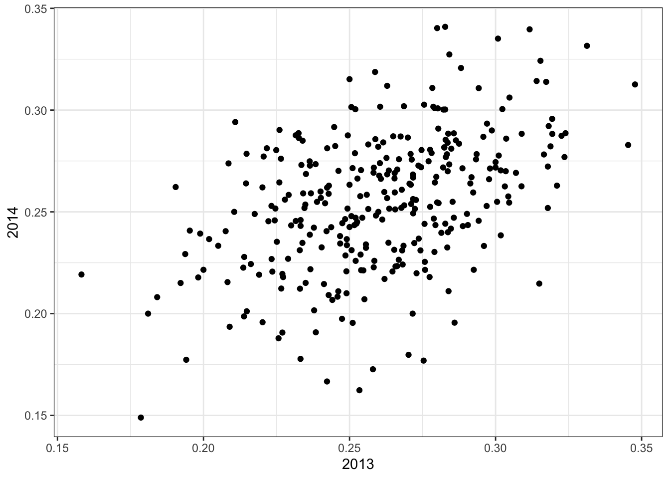

summarize(two_years, cor(`2013`,`2014`))

## # A tibble: 1 x 1
##   `cor(\`2013\`, \`2014\`)`
##                       <dbl>
## 1                     0.460

3.22 Measurement Error Models

The textbook for this section is available here

Key points

Up to now, all our linear regression examples have been applied to two or more random variables. We assume the pairs are bivariate normal and use this to motivate a linear model.
Another use for linear regression is with measurement error models, where it is common to have a non-random covariate (such as time). Randomness is introduced from measurement error rather than sampling or natural variability.

Code

The code to use dslabs function rfalling_object to generate simulations of dropping balls:

falling_object <- rfalling_object()

The code to draw the trajectory of the ball:

falling_object %>%
    ggplot(aes(time, observed_distance)) +
    geom_point() +
    ylab("Distance in meters") +
    xlab("Time in seconds")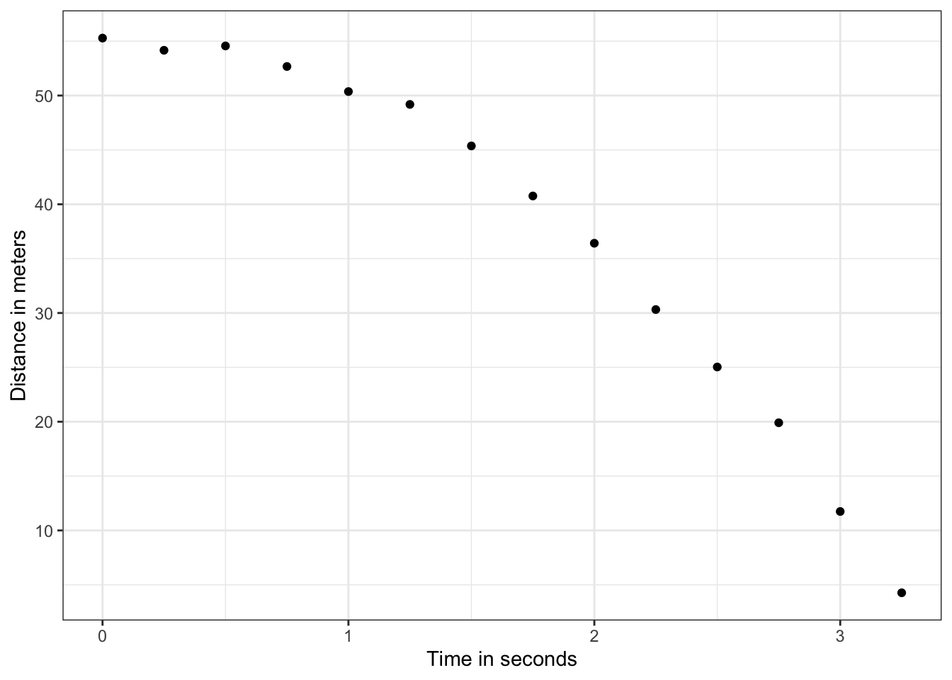

The code to use the lm() function to estimate the coefficients:

fit <- falling_object %>%
    mutate(time_sq = time^2) %>%
    lm(observed_distance~time+time_sq, data=.)

tidy(fit)

## # A tibble: 3 x 5
##   term        estimate std.error statistic  p.value
##   <chr>          <dbl>     <dbl>     <dbl>    <dbl>
## 1 (Intercept)   55.0       0.434    127.   9.15e-19
## 2 time           0.888     0.620      1.43 1.80e- 1
## 3 time_sq       -5.08      0.184    -27.7  1.61e-11

The code to check if the estimated parabola fits the data:

augment(fit) %>%
    ggplot() +
    geom_point(aes(time, observed_distance)) +
    geom_line(aes(time, .fitted), col = "blue")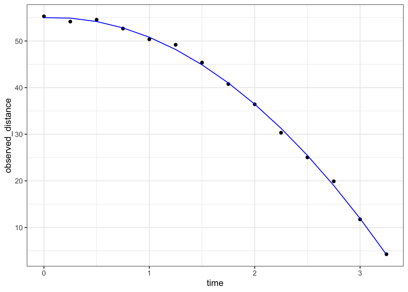

The code to see the summary statistic of the regression:

tidy(fit, conf.int = TRUE)

## # A tibble: 3 x 7
##   term        estimate std.error statistic  p.value conf.low conf.high
##   <chr>          <dbl>     <dbl>     <dbl>    <dbl>    <dbl>     <dbl>
## 1 (Intercept)   55.0       0.434    127.   9.15e-19   54.1       56.0 
## 2 time           0.888     0.620      1.43 1.80e- 1   -0.476      2.25
## 3 time_sq       -5.08      0.184    -27.7  1.61e-11   -5.49      -4.68

3.23 Assessment - Regression and Baseball, part 1

What is the final linear model (in the video “Building a Better Offensive Metric for Baseball”) we used to predict runs scored per game?

A. lm(R ~ BB + HR)
B. lm(HR ~ BB + singles + doubles + triples)
C. lm(R ~ BB + singles + doubles + triples + HR)
D. lm(R ~ singles + doubles + triples + HR)

We want to estimate runs per game scored by individual players, not just by teams. What summary metric do we calculate to help estimate this?

Look at the code from the video “Building a Metter Offensive Metric for Baseball” for a hint:

pa_per_game <- Batting %>% 
  filter(yearID == 2002) %>% 
  group_by(teamID) %>%
  summarize(pa_per_game = sum(AB+BB)/max(G)) %>% 
  .$pa_per_game %>% 
  mean

A. pa_per_game: the mean number of plate appearances per team per game for each team
B. pa_per_game: the mean number of plate appearances per game for each player
C. pa_per_game: the number of plate appearances per team per game, averaged across all teams

Imagine you have two teams. Team A is comprised of batters who, on average, get two bases on balls, four singles, one double, and one home run. Team B is comprised of batters who, on average, get one base on balls, six singles, two doubles, and one triple.

Which team scores more runs, as predicted by our model?

A. Team A
B. Team B
C. Tie
D. Impossible to know

The on-base-percentage plus slugging percentage (OPS) metric gives the most weight to:

A. Singles
B. Doubles
C. Triples
D. Home Runs

What statistical concept properly explains the “sophomore slump”?

A. Regression to the mean
B. Law of averages
C. Normal distribution

In our model of time vs. observed_distance in the video “Measurement Error Models”, the randomness of our data was due to:

A. sampling
B. natural variability
C. measurement error

Which of the following are important assumptions about the measurement errors in this experiment?

A. The measurement error is random
B. The measurement error is independent
C. The measurement error has the same distribution for each time i

Which of the following scenarios would violate an assumption of our measurement error model?

A. The experiment was conducted on the moon.
B. There was one position where it was particularly difficult to see the dropped ball.
C. The experiment was only repeated 10 times, not 100 times.

3.24 Assessment - Regression and Baseball, part 2

Question 9 has two parts. Use the information below to answer both parts.

Use the Teams data frame from the Lahman package. Fit a multivariate linear regression model to obtain the effects of BB and HR on Runs (R) in 1971. Use the tidy() function in the broom package to obtain the results in a data frame.

9a. What is the estimate for the effect of BB on runs?

Teams %>%
    filter(yearID == 1971) %>%
    lm(R ~ BB + HR, data = .) %>%
    tidy() %>%
    filter(term == "BB") %>%
    pull(estimate)

## [1] 0.414

What is the estimate for the effect of HR on runs?

Teams %>%
    filter(yearID == 1971) %>%
    lm(R ~ BB + HR, data = .) %>%
    tidy() %>%
    filter(term == "HR") %>%
    pull(estimate)

## [1] 1.3

9b. Interpret the p-values for the estimates using a cutoff of 0.05.

Which of the following is the correct interpretation?

fit <- Teams %>% filter(yearID %in% 1971) %>% 
mutate(BB = BB/G, HR = HR/G,  R = R/G) %>%  
lm(R ~ BB + HR, data = .)

tidy(fit, conf.int = TRUE)

## # A tibble: 3 x 7
##   term        estimate std.error statistic p.value conf.low conf.high
##   <chr>          <dbl>     <dbl>     <dbl>   <dbl>    <dbl>     <dbl>
## 1 (Intercept)    1.60      0.665      2.40 0.0256    0.215      2.98 
## 2 BB             0.412     0.203      2.03 0.0552   -0.0101     0.835
## 3 HR             1.29      0.427      3.03 0.00639   0.406      2.18

A. Both BB and HR have a nonzero effect on runs.
B. HR has a significant effect on runs, but the evidence is not strong enough to suggest BB also does.
C. BB has a significant effect on runs, but the evidence is not strong enough to suggest HR also does.
D. Neither BB nor HR have a statistically significant effect on runs.

Repeat the above exercise to find the effects of BB and HR on runs (R) for every year from 1961 to 2018 using do() and the broom package.

Make a scatterplot of the estimate for the effect of BB on runs over time and add a trend line with confidence intervals.

res <- Teams %>%
    filter(yearID %in% 1961:2018) %>%
    group_by(yearID) %>%
    do(tidy(lm(R ~ BB + HR, data = .))) %>%
    ungroup() 
res %>%
    filter(term == "BB") %>%
    ggplot(aes(yearID, estimate)) +
    geom_point() +
    geom_smooth(method = "lm")

## `geom_smooth()` using formula 'y ~ x'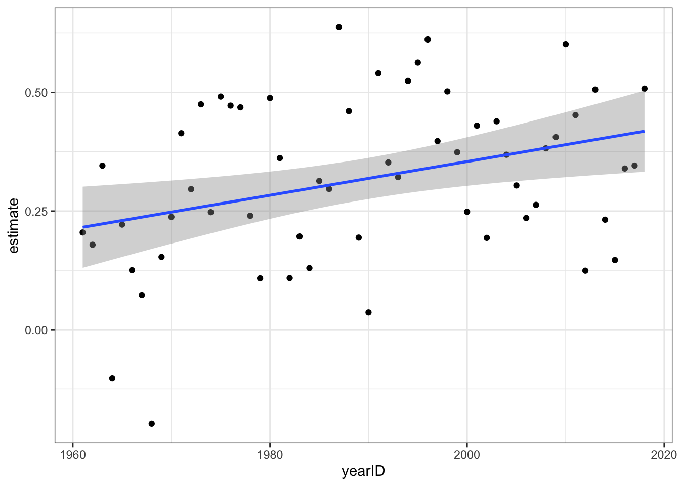

Fill in the blank to complete the statement:

The effect of BB on runs has increased over time.

Fit a linear model on the results from Question 10 to determine the effect of year on the impact of BB.

For each additional year, by what value does the impact of BB on runs change?

res %>%
    filter(term == "BB") %>%
    lm(estimate ~ yearID, data = .) %>%
    tidy() %>%
    filter(term == "yearID") %>%
    pull(estimate)

## [1] 0.00355

What is the p-value for this effect?

res %>%
    filter(term == "BB") %>%
    lm(estimate ~ yearID, data = .) %>%
    tidy() %>%
    filter(term == "yearID") %>%
    pull(p.value)

## [1] 0.00807

3.25 Assessment - Linear Models

This assessment has 6 multi-part questions that will all use the setup below.

Game attendance in baseball varies partly as a function of how well a team is playing.

Load the Lahman library. The Teams data frame contains an attendance column. This is the total attendance for the season. To calculate average attendance, divide by the number of games played, as follows:

Teams_small <- Teams %>% 
    filter(yearID %in% 1961:2001) %>% 
    mutate(avg_attendance = attendance/G)

Use linear models to answer the following 3-part question about Teams_small.

1a. Use runs (R) per game to predict average attendance.

For every 1 run scored per game, average attendance increases by how much?

# find regression line predicting attendance from R and take slope
Teams_small %>% 
  mutate(R_per_game = R/G) %>% 
  lm(avg_attendance ~ R_per_game, data = .) %>% 
  .$coef %>%
  .[2]

## R_per_game 
##       4117

Use home runs (HR) per game to predict average attendance.

For every 1 home run hit per game, average attendance increases by how much?

Teams_small %>% 
  mutate(HR_per_game = HR/G) %>% 
  lm(avg_attendance ~ HR_per_game, data = .) %>% 
  .$coef %>%
  .[2]

## HR_per_game 
##        8113

1b. Use number of wins to predict average attendance; do not normalize for number of games.

For every game won in a season, how much does average attendance increase?

Teams_small %>% 
  lm(avg_attendance ~ W, data = .) %>%
  .$coef %>%
  .[2]

##   W 
## 121

Suppose a team won zero games in a season.

Predict the average attendance.

Teams_small %>% 
  lm(avg_attendance ~ W, data = .) %>% 
  .$coef %>%
  .[1]

## (Intercept) 
##        1129

1c. Use year to predict average attendance.

How much does average attendance increase each year?

Teams_small %>% 
  lm(avg_attendance ~ yearID, data = .) %>% 
  .$coef %>%
  .[2]

## yearID 
##    244

Game wins, runs per game and home runs per game are positively correlated with attendance. We saw in the course material that runs per game and home runs per game are correlated with each other. Are wins and runs per game or wins and home runs per game correlated?

What is the correlation coefficient for wins and runs per game?

cor(Teams_small$W, Teams_small$R/Teams_small$G)

## [1] 0.412

What is the correlation coefficient for wins and home runs per game?

cor(Teams_small$W, Teams_small$HR/Teams_small$G)

## [1] 0.274

Stratify Teams_small by wins: divide number of wins by 10 and then round to the nearest integer. Keep only strata 5 through 10, which have 20 or more data points.

Use the stratified dataset to answer this three-part question.

3a. How many observations are in the 8 win strata? (Note that due to division and rounding, these teams have 75-85 wins.)

dat <- Teams_small %>%
    mutate(W_strata = round(W/10)) %>%
    filter(W_strata >= 5 & W_strata <= 10)

sum(dat$W_strata == 8)

## [1] 338

3b. Calculate the slope of the regression line predicting average attendance given runs per game for each of the win strata.

Which win stratum has the largest regression line slope?

# calculate slope of regression line after stratifying by R per game
dat %>%  
  group_by(W_strata) %>%
  summarize(slope = cor(R/G, avg_attendance)*sd(avg_attendance)/sd(R/G))

## `summarise()` ungrouping output (override with `.groups` argument)

## # A tibble: 6 x 2
##   W_strata slope
##      <dbl> <dbl>
## 1        5 4362.
## 2        6 4343.
## 3        7 3888.
## 4        8 3128.
## 5        9 3701.
## 6       10 3107.

Calculate the slope of the regression line predicting average attendance given HR per game for each of the win strata.

Which win stratum has the largest regression line slope?

# calculate slope of regression line after stratifying by HR per game
dat %>%  
  group_by(W_strata) %>%
  summarize(slope = cor(HR/G, avg_attendance)*sd(avg_attendance)/sd(HR/G))

## `summarise()` ungrouping output (override with `.groups` argument)

## # A tibble: 6 x 2
##   W_strata  slope
##      <dbl>  <dbl>
## 1        5 10192.
## 2        6  7032.
## 3        7  8931.
## 4        8  6301.
## 5        9  5863.
## 6       10  4917.

3c. Which of the followng are true about the effect of win strata on average attendance?

A. Across all win strata, runs per game are positively correlated with average attendance.
B. Runs per game have the strongest effect on attendance when a team wins many games.
C. After controlling for number of wins, home runs per game are not correlated with attendance.
D. Home runs per game have the strongest effect on attendance when a team does not win many games.
E. Among teams with similar numbers of wins, teams with more home runs per game have larger average attendance.

Fit a multivariate regression determining the effects of runs per game, home runs per game, wins, and year on average attendance. Use the original Teams_small wins column, not the win strata from question 3.

What is the estimate of the effect of runs per game on average attendance?

fit <- Teams_small %>% 
    mutate(R_per_game = R/G,
           HR_per_game = HR/G) %>%
    lm(avg_attendance ~ R_per_game + HR_per_game + W + yearID, data = .)
tidy(fit) %>%
    filter(term == "R_per_game") %>%
    pull(estimate)

## [1] 322

What is the estimate of the effect of home runs per game on average attendance?

tidy(fit) %>%
    filter(term == "HR_per_game") %>%
    pull(estimate)

## [1] 1798

What is the estimate of the effect of number of wins in a season on average attendance?

tidy(fit) %>%
    filter(term == "W") %>%
    pull(estimate)

## [1] 117

Use the multivariate regression model from Question 4. Suppose a team averaged 5 runs per game, 1.2 home runs per game, and won 80 games in a season.

What would this team’s average attendance be in 2002?

predict(fit, data.frame(R_per_game = 5, HR_per_game = 1.2, W = 80, yearID = 2002))

##     1 
## 16149

What would this team’s average attendance be in 1960?

predict(fit, data.frame(R_per_game = 5, HR_per_game = 1.2, W = 80, yearID = 1960))

##    1 
## 6505

Use your model from Question 4 to predict average attendance for teams in 2002 in the original Teams data frame.

What is the correlation between the predicted attendance and actual attendance?

newdata <- Teams %>%
    filter(yearID == 2002) %>%
    mutate(avg_attendance = attendance/G,
           R_per_game = R/G,
           HR_per_game = HR/G)
preds <- predict(fit, newdata)
cor(preds, newdata$avg_attendance)

## [1] 0.519