2 Section 1 Overview
Section 1 introduces you to Discrete Probability. Section 1 is divided into three parts:
- Introduction to Discrete Probability
- Combinations and Permutations
- Addition Rule and Monty Hall
After completing Section 1, you will be able to:
- Apply basic probability theory to categorical data.
- Perform a Monte Carlo simulation to approximate the results of repeating an experiment over and over, including simulating the outcomes in the Monty Hall problem.
- Distinguish between: sampling with and without replacement, events that are and are not independent, and combinations and permutations.
- Apply the multiplication and addition rules, as appropriate, to calculate the probably of multiple events occurring.
- Use sapply instead of a for loop to perform element-wise operations on a function.
2.1 Discrete Probability
The textbook for this section is available here.
Key points
- The probability of an event is the proportion of times the event occurs when we repeat the experiment independently under the same conditions.
\(\mbox{Pr}(A)\) = probability of event A
- An event is defined as an outcome that can occur when when something happens by chance.
- We can determine probabilities related to discrete variables (picking a red bead, choosing 48 Democrats and 52 Republicans from 100 likely voters) and continuous variables (height over 6 feet).
2.2 Monte Carlo Simulations
The textbook for this section is available here.
Key points
- Monte Carlo simulations model the probability of different outcomes by repeating a random process a large enough number of times that the results are similar to what would be observed if the process were repeated forever.
- The sample function draws random outcomes from a set of options.
- The replicate function repeats lines of code a set number of times. It is used with sample and similar functions to run Monte Carlo simulations.
Code: The rep function and the sample function
beads <- rep(c("red", "blue"), times = c(2,3))    # create an urn with 2 red, 3 blue
beads    # view beads object
## [1] "red" "red" "blue" "blue" "blue"sample(beads, 1) # sample 1 bead at random## [1] "red"Code: Monte Carlo simulation
Note that your exact outcome values will differ because the sampling is random.
B <- 10000    # number of times to draw 1 bead
events <- replicate(B, sample(beads, 1))    # draw 1 bead, B times
tab <- table(events)    # make a table of outcome counts
tab    # view count table
## events
## blue red
## 6004 3996prop.table(tab) # view table of outcome proportions## events
## blue red
## 0.6004 0.39962.3 Setting the Random Seed
The set.seed function
Before we continue, we will briefly explain the following important line of code:
set.seed(1986)Throughout this book, we use random number generators. This implies that many of the results presented can actually change by chance, which then suggests that a frozen version of the book may show a different result than what you obtain when you try to code as shown in the book. This is actually fine since the results are random and change from time to time. However, if you want to to ensure that results are exactly the same every time you run them, you can set R’s random number generation seed to a specific number. Above we set it to 1986. We want to avoid using the same seed every time. A popular way to pick the seed is the year - month - day. For example, we picked 1986 on December 20, 2018: 2018 − 12 − 20 = 1986.
You can learn more about setting the seed by looking at the documentation:
?set.seedIn the exercises, we may ask you to set the seed to assure that the results you obtain are exactly what we expect them to be.
Important note on seeds in R 3.5 and R 3.6
R was updated to version 3.6 in early 2019. In this update, the default method for setting the seed changed. This means that exercises, videos, textbook excerpts and other code you encounter online may yield a different result based on your version of R.
If you are running R 3.6, you can revert to the original seed setting behavior by adding the argument sample.kind=“Rounding”. For example:
set.seed(1)
set.seed(1, sample.kind="Rounding")    # will make R 3.6 generate a seed as in R 3.5
Using the sample.kind="Rounding" argument will generate a message:
non-uniform 'Rounding' sampler used
This is not a warning or a cause for alarm - it is a confirmation that R is using the alternate seed generation method, and you should expect to receive this message in your console.
If you use R 3.6, you should always use the second form of set.seed in this course series (outside of DataCamp assignments). Failure to do so may result in an otherwise correct answer being rejected by the grader. In most cases where a seed is required, you will be reminded of this fact.
2.4 Using the mean Function for Probability
An important application of the mean function
In R, applying the mean function to a logical vector returns the proportion of elements that are TRUE. It is very common to use the mean function in this way to calculate probabilities and we will do so throughout the course.
Suppose you have the vector beads:
beads <- rep(c("red", "blue"), times = c(2,3))
beads
## [1] "red" "red" "blue" "blue" "blue"# To find the probability of drawing a blue bead at random, you can run:
mean(beads == "blue")## [1] 0.6This code is broken down into steps inside R. First, R evaluates the logical statement beads == "blue", which generates the vector:
FALSE FALSE TRUE TRUE TRUE
When the mean function is applied, R coerces the logical values to numeric values, changing TRUE to 1 and FALSE to 0:
0 0 1 1 1
The mean of the zeros and ones thus gives the proportion of TRUE values. As we have learned and will continue to see, probabilities are directly related to the proportion of events that satisfy a requirement.
2.5 Probability Distributions
The textbook for this section is available here.
Key points
- The probability distribution for a variable describes the probability of observing each possible outcome.
- For discrete categorical variables, the probability distribution is defined by the proportions for each group.
2.6 Independence
The textbook section on independence, conditional probability and the multiplication rule is available here.
Key points
- Conditional probabilities compute the probability that an event occurs given information about dependent events. For example, the probability of drawing a second king given that the first draw is a king is:
\(\mbox{Pr}(\text{Card 2 is a king} \mid \text{Card 1 is a king}) = 3/51\)
- If two events \(A\) and \(B\) are independent, \(\mbox{Pr}(A \mid B) = \mbox{Pr}(A)\).
- To determine the probability of multiple events occurring, we use the multiplication rule.
Equations
The multiplication rule for independent events is:
\(\mbox{Pr}(\text{A and B and C}) = \mbox{Pr}(A)\:X\:\mbox{Pr}(B)\:X\:\mbox{Pr}(C)\)
The multiplication rule for dependent events considers the conditional probability of both events occurring:
\(\mbox{Pr}(\text{A and B}) = \mbox{Pr}(A)\:X\:\mbox{Pr}(B \mid A)\)
We can expand the multiplication rule for dependent events to more than 2 events:
\(\mbox{Pr}(\text{A and B and C}) = \mbox{Pr}(A)\:X\:\mbox{Pr}(B \mid A)\:X\:\mbox{Pr}(C \mid \text{A and B})\)
2.7 Assessment - Introduction to Discrete Probability (using R)
- Probability of cyan
One ball will be drawn at random from a box containing: 3 cyan balls, 5 magenta balls, and 7 yellow balls.
What is the probability that the ball will be cyan?
cyan <- 3
magenta <- 5
yellow <- 7

# Assign a variable `p` as the probability of choosing a cyan ball from the box
p <- cyan/(cyan+magenta+yellow)

# Print the variable `p` to the console
p
## [1] 0.2- Probability of not cyan
One ball will be drawn at random from a box containing: 3 cyan balls, 5 magenta balls, and 7 yellow balls.
What is the probability that the ball will not be cyan?
# `p` is defined as the probability of choosing a cyan ball from a box containing: 3 cyan balls, 5 magenta balls, and 7 yellow balls.
# Using variable `p`, calculate the probability of choosing any ball that is not cyan from the box
p <- cyan/(cyan+magenta+yellow)
prop <- 1 - p
prop
## [1] 0.8- Sampling without replacement
Instead of taking just one draw, consider taking two draws. You take the second draw without returning the first draw to the box. We call this sampling without replacement.
What is the probability that the first draw is cyan and that the second draw is not cyan?
# The variable `p_1` is the probability of choosing a cyan ball from the box on the first draw.
p_1 <- cyan / (cyan + magenta + yellow)

# Assign a variable `p_2` as the probability of not choosing a cyan ball on the second draw without replacement.
p_2 <- (magenta+yellow)/((cyan-1)+magenta+yellow)
p_2
## [1] 0.8571429# Calculate the probability that the first draw is cyan and the second draw is not cyan using `p_1` and `p_2`.
p_1 * p_2## [1] 0.1714286- Sampling with replacement
Now repeat the experiment, but this time, after taking the first draw and recording the color, return it back to the box and shake the box. We call this sampling with replacement. What is the probability that the first draw is cyan and that the second draw is not cyan?
# The variable 'p_1' is the probability of choosing a cyan ball from the box on the first draw.
p_1 <- cyan / (cyan + magenta + yellow)
# Assign a variable 'p_2' as the probability of not choosing a cyan ball on the second draw with replacement.
p_2 <- (magenta + yellow) / (cyan + magenta + yellow)
# Calculate the probability that the first draw is cyan and the second draw is not cyan using `p_1` and `p_2`.
p_1 * p_2
## [1] 0.162.8 Combinations and Permutations
The textbook for this section is available here.
Key points
- paste joins two strings and inserts a space in between.
- expand.grid gives the combinations of 2 vectors or lists.
- permutations(n,r) from the gtools package lists the different ways that r items can be selected from a set of n options when order matters.
- combinations(n,r) from the gtools package lists the different ways that r items can be selected from a set of n options when order does not matter.
Code: Introducing paste and expand.grid
# joining strings with paste
number <- "Three"
suit <- "Hearts"
paste(number, suit)
## [1] "Three Hearts"# joining vectors element-wise with paste
paste(letters[1:5], as.character(1:5))## [1] "a 1" "b 2" "c 3" "d 4" "e 5"# generating combinations of 2 vectors with expand.grid
expand.grid(pants = c("blue", "black"), shirt = c("white", "grey", "plaid"))## pants shirt
## 1 blue white
## 2 black white
## 3 blue grey
## 4 black grey
## 5 blue plaid
## 6 black plaidCode: Generating a deck of cards
suits <- c("Diamonds", "Clubs", "Hearts", "Spades")
numbers <- c("Ace", "Deuce", "Three", "Four", "Five", "Six", "Seven", "Eight", "Nine", "Ten", "Jack", "Queen", "King")
deck <- expand.grid(number = numbers, suit = suits)
deck <- paste(deck$number, deck$suit)

# probability of drawing a king
kings <- paste("King", suits)
mean(deck %in% kings)
## [1] 0.07692308Code: Permutations and combinations
if(!require(gtools)) install.packages("gtools")## Loading required package: gtoolslibrary(gtools)
permutations(5,2) # ways to choose 2 numbers in order from 1:5## [,1] [,2]
## [1,] 1 2
## [2,] 1 3
## [3,] 1 4
## [4,] 1 5
## [5,] 2 1
## [6,] 2 3
## [7,] 2 4
## [8,] 2 5
## [9,] 3 1
## [10,] 3 2
## [11,] 3 4
## [12,] 3 5
## [13,] 4 1
## [14,] 4 2
## [15,] 4 3
## [16,] 4 5
## [17,] 5 1
## [18,] 5 2
## [19,] 5 3
## [20,] 5 4all_phone_numbers <- permutations(10, 7, v = 0:9)
n <- nrow(all_phone_numbers)
index <- sample(n, 5)
all_phone_numbers[index,]## [,1] [,2] [,3] [,4] [,5] [,6] [,7]
## [1,] 1 4 7 8 3 6 0
## [2,] 2 7 0 1 4 8 6
## [3,] 4 2 5 3 7 8 1
## [4,] 7 0 8 6 2 5 1
## [5,] 4 0 8 5 3 6 7permutations(3,2) # order matters## [,1] [,2]
## [1,] 1 2
## [2,] 1 3
## [3,] 2 1
## [4,] 2 3
## [5,] 3 1
## [6,] 3 2combinations(3,2) # order does not matter## [,1] [,2]
## [1,] 1 2
## [2,] 1 3
## [3,] 2 3Code: Probability of drawing a second king given that one king is drawn
hands <- permutations(52,2, v = deck)
first_card <- hands[,1]
second_card <- hands[,2]
sum(first_card %in% kings)
## [1] 204sum(first_card %in% kings & second_card %in% kings) / sum(first_card %in% kings)## [1] 0.05882353Code: Probability of a natural 21 in blackjack
aces <- paste("Ace", suits)

facecard <- c("King", "Queen", "Jack", "Ten")
facecard <- expand.grid(number = facecard, suit = suits)
facecard <- paste(facecard$number, facecard$suit)

hands <- combinations(52, 2, v=deck) # all possible hands

# probability of a natural 21 given that the ace is listed first in `combinations`
mean(hands[,1] %in% aces & hands[,2] %in% facecard)
## [1] 0.04826546# probability of a natural 21 checking for both ace first and ace second
mean((hands[,1] %in% aces & hands[,2] %in% facecard)|(hands[,2] %in% aces & hands[,1] %in% facecard))## [1] 0.04826546Code: Monte Carlo simulation of natural 21 in blackjack
Note that your exact values will differ because the process is random and the seed is not set.
# code for one hand of blackjack
hand <- sample(deck, 2)
hand
## [1] "Jack Hearts" "Five Diamonds"# code for B=10,000 hands of blackjack
B <- 10000
results <- replicate(B, {
hand <- sample(deck, 2)
(hand[1] %in% aces & hand[2] %in% facecard) | (hand[2] %in% aces & hand[1] %in% facecard)
})
mean(results)## [1] 0.05042.9 The Birthday Problem
The textbook for this section is available here.
Key points
- duplicated takes a vector and returns a vector of the same length with TRUE for any elements that have appeared previously in that vector.
- We can compute the probability of shared birthdays in a group of people by modeling birthdays as random draws from the numbers 1 through 365. We can then use this sampling model of birthdays to run a Monte Carlo simulation to estimate the probability of shared birthdays.
Code: The birthday problem
# checking for duplicated bdays in one 50 person group
n <- 50
bdays <- sample(1:365, n, replace = TRUE)    # generate n random birthdays
any(duplicated(bdays))    # check if any birthdays are duplicated
## [1] TRUE# Monte Carlo simulation with B=10000 replicates
B <- 10000
results <- replicate(B, { # returns vector of B logical values
bdays <- sample(1:365, n, replace = TRUE)
any(duplicated(bdays))
})
mean(results) # calculates proportion of groups with duplicated bdays## [1] 0.96952.10 sapply
The textbook discussion of the basics of sapply can be found in this textbook section.
The textbook discussion of sapply for the birthday problem can be found within the birthday problem section.
Key points
- Some functions automatically apply element-wise to vectors, such as sqrt and *****.
- However, other functions do not operate element-wise by default. This includes functions we define ourselves.
- The function sapply(x, f) allows any other function f to be applied element-wise to the vector x.
- The probability of an event happening is 1 minus the probability of that event not happening:
\(\mbox{Pr}(event) = 1 - \mbox{Pr}(\text{no event})\)
- We can compute the probability of shared birthdays mathematically:
\(\mbox{Pr}(\text{shared birthdays}) = 1 − \mbox{Pr}(\text{no shared birthdays}) = 1 − (1\:X\: \frac{364}{365}\:X \:\frac{363}{365}\:X...X\: \frac{365−n+1}{365})\)
Code: Function for calculating birthday problem Monte Carlo simulations for any value of n
Note that the function body of compute_prob is the code that we wrote earlier. If we write this code as a function, we can use sapply to apply this function to several values of n.
# function to calculate probability of shared bdays across n people
compute_prob <- function(n, B = 10000) {
    same_day <- replicate(B, {
        bdays <- sample(1:365, n, replace = TRUE)
        any(duplicated(bdays))
    })
    mean(same_day)
}

n <- seq(1, 60)
Code: Element-wise operation over vectors and sapply
x <- 1:10
sqrt(x)    # sqrt operates on each element of the vector
## [1] 1.000000 1.414214 1.732051 2.000000 2.236068 2.449490 2.645751 2.828427 3.000000 3.162278y <- 1:10
x*y # * operates element-wise on both vectors## [1] 1 4 9 16 25 36 49 64 81 100compute_prob(n) # does not iterate over the vector n without sapply## [1] 0x <- 1:10
sapply(x, sqrt) # this is equivalent to sqrt(x)## [1] 1.000000 1.414214 1.732051 2.000000 2.236068 2.449490 2.645751 2.828427 3.000000 3.162278prob <- sapply(n, compute_prob) # element-wise application of compute_prob to n
plot(n, prob)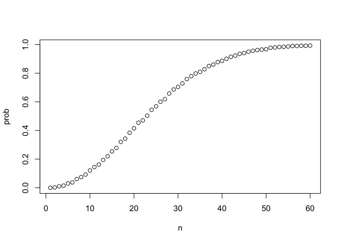
Computing birthday problem probabilities with sapply
# function for computing exact probability of shared birthdays for any n
exact_prob <- function(n){
    prob_unique <- seq(365, 365-n+1)/365   # vector of fractions for mult. rule
    1 - prod(prob_unique)    # calculate prob of no shared birthdays and subtract from 1
}

# applying function element-wise to vector of n values
eprob <- sapply(n, exact_prob)

# plotting Monte Carlo results and exact probabilities on same graph
plot(n, prob)    # plot Monte Carlo results
lines(n, eprob, col = "red")    # add line for exact prob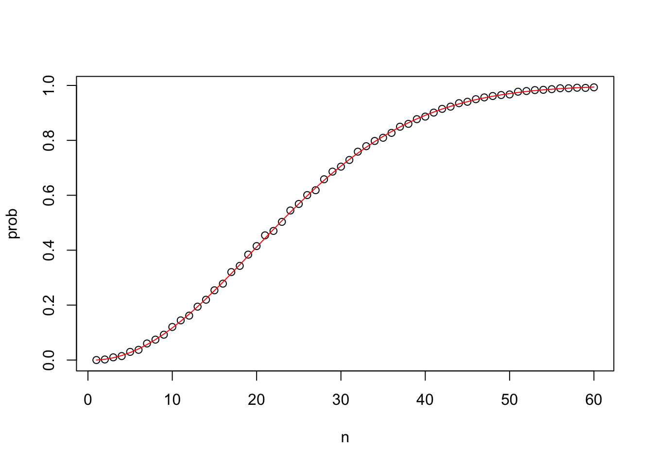
2.11 How many Monte Carlo Experiments are enough?
Here is a link to the matching textbook section.
Key points
- The larger the number of Monte Carlo replicates \(B\), the more accurate the estimate.
- Determining the appropriate size for \(B\) can require advanced statistics.
- One practical approach is to try many sizes for \(B\) and look for sizes that provide stable estimates.
Code: Estimating a practical value of B
This code runs Monte Carlo simulations to estimate the probability of shared birthdays using several B values and plots the results. When B is large enough that the estimated probability stays stable, then we have selected a useful value of B.
B <- 10^seq(1, 5, len = 100)    # defines vector of many B values
compute_prob <- function(B, n = 22){    # function to run Monte Carlo simulation with each B
    same_day <- replicate(B, {
        bdays <- sample(1:365, n, replace = TRUE)
        any(duplicated(bdays))
    })
    mean(same_day)
}
prob <- sapply(B, compute_prob)    # apply compute_prob to many values of B
plot(log10(B), prob, type = "l")    # plot a line graph of estimates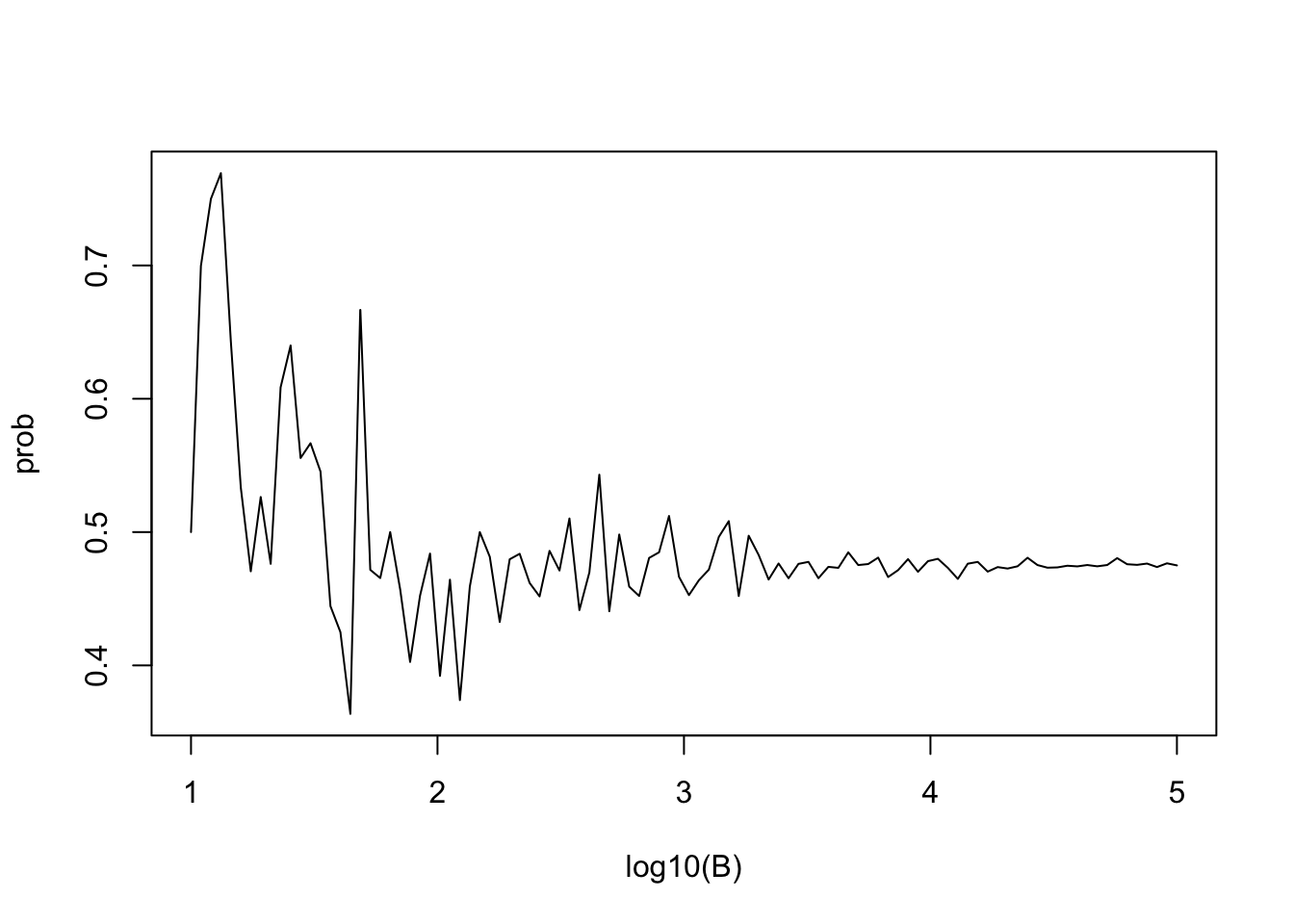
2.12 Assessment - Combinations and Permutations
1.Imagine you draw two balls from a box containing colored balls. You either replace the first ball before you draw the second or you leave the first ball out of the box when you draw the second ball.
Under which situation are the two draws independent of one another?
Remember that two events A and B are independent if:
\(\mbox{Pr}(\text{A and B}) = \mbox{Pr}(A)P(B)\)
- A. You don’t replace the first ball before drawing the next.
- B. You do replace the first ball before drawing the next.
- C. Neither situation describes independent events.
- D. Both situations describe independent events.
- Say you’ve drawn 5 balls from the a box that has 3 cyan balls, 5 magenta balls, and 7 yellow balls, with replacement, and all have been yellow.
What is the probability that the next one is yellow?
# Assign the variable 'p_yellow' as the probability that a yellow ball is drawn from the box.
p_yellow <- yellow / (cyan + magenta + yellow)

# Using the variable 'p_yellow', calculate the probability of drawing a yellow ball on the sixth draw. Print this value to the console.
p_yellow
## [1] 0.4666667- If you roll a 6-sided die once, what is the probability of not seeing a 6? If you roll a 6-sided die six times, what is the probability of not seeing a 6 on any roll?
# Assign the variable 'p_no6' as the probability of not seeing a 6 on a single roll.
p_no6 <- 5/6

# Calculate the probability of not seeing a 6 on six rolls using `p_no6`. Print your result to the console: do not assign it to a variable.
p_no6*p_no6*p_no6*p_no6*p_no6*p_no6
## [1] 0.334898- Two teams, say the Celtics and the Cavs, are playing a seven game series. The Cavs are a better team and have a 60% chance of winning each game.
What is the probability that the Celtics win at least one game? Remember that the Celtics must win one of the first four games, or the series will be over!
# Assign the variable `p_cavs_win4` as the probability that the Cavs will win the first four games of the series.
p_cavs_win4 <- (3/5)*(3/5)*(3/5)*(3/5)

# Using the variable `p_cavs_win4`, calculate the probability that the Celtics win at least one game in the first four games of the series.
1-p_cavs_win4
## [1] 0.8704- Create a Monte Carlo simulation to confirm your answer to the previous problem by estimating how frequently the Celtics win at least 1 of 4 games. Use
B <- 10000simulations.
The provided sample code simulates a single series of four random games, simulated_games
# This line of example code simulates four independent random games where the Celtics either lose or win. Copy this example code to use within the `replicate` function.
simulated_games <- sample(c("lose","win"), 4, replace = TRUE, prob = c(0.6, 0.4))

# The variable 'B' specifies the number of times we want the simulation to run. Let's run the Monte Carlo simulation 10,000 times.
B <- 10000

# Use the `set.seed` function to make sure your answer matches the expected result after random sampling.
set.seed(1)

# Create an object called `celtic_wins` that replicates two steps for B iterations: (1) generating a random four-game series `simulated_games` using the example code, then (2) determining whether the simulated series contains at least one win for the Celtics.
celtic_wins <- replicate(B, {
  simulated_games <- sample(c("lose","win"), 4, replace = TRUE, prob = c(0.6, 0.4))
  any(simulated_games=="win")}
)

# Calculate the frequency out of B iterations that the Celtics won at least one game. Print your answer to the console.
mean(celtic_wins)
## [1] 0.87572.13 The Addition rule
Here is a link to the textbook section on the addition rule.
Key points
- The addition rule states that the probability of event \(A\) or event \(B\) happening is the probability of event \(A\) plus the probability of event \(B\) minus the probability of both events \(A\) and \(B\) happening together.
\(\mbox{Pr}(\text{A or B})=\mbox{Pr}(A) + \mbox{Pr}(B) − \mbox{Pr}(\text{A and B})\)
Note that \((\text{A or B})\) is equivalent to \((A \mid B)\).
Example: The addition rule for a natural 21 in blackjack
We apply the addition rule where \(A\) = drawing an ace then a facecard and \(B\) = drawing a facecard then an ace. Note that in this case, both events A and B cannot happen at the same time, so \(\mbox{Pr}(\text{A and B}) = 0\).
\(\mbox{Pr}(\text{ace then facecard}) = \frac{4}{52}\:X\: \frac{16}{51}\)
\(\mbox{Pr}(\text{facecard then ace}) = \frac{16}{52}\:X\: \frac{4}{51}\)
\(\mbox{Pr}(\text{ace then facecard} \mid \text{facecard then ace}) = \frac{4}{52}\:X\: \frac{16}{51} + \frac{16}{52}\:X\: \frac{4}{51} = 0.0483\)
2.14 The Monty Hall Problem
Here is the textbook section on the Monty Hall Problem.
Key points
- Monte Carlo simulations can be used to simulate random outcomes, which makes them useful when exploring ambiguous or less intuitive problems like the Monty Hall problem.
- In the Monty Hall problem, contestants choose one of three doors that may contain a prize. Then, one of the doors that was not chosen by the contestant and does not contain a prize is revealed. The contestant can then choose whether to stick with the original choice or switch to the remaining unopened door.
- Although it may seem intuitively like the contestant has a 1 in 2 chance of winning regardless of whether they stick or switch, Monte Carlo simulations demonstrate that the actual probability of winning is 1 in 3 with the stick strategy and 2 in 3 with the switch strategy.
- For more on the Monty Hall problem, you can watch a detailed explanation here or read an explanation here.
Code: Monte Carlo simulation of stick strategy
B <- 10000
stick <- replicate(B, {
  doors <- as.character(1:3)
  prize <- sample(c("car","goat","goat"))    # puts prizes in random order
  prize_door <- doors[prize == "car"]    # note which door has prize
  my_pick  <- sample(doors, 1)    # note which door is chosen
  show <- sample(doors[!doors %in% c(my_pick, prize_door)],1)    # open door with no prize that isn't chosen
  stick <- my_pick    # stick with original door
  stick == prize_door    # test whether the original door has the prize
})
mean(stick)    # probability of choosing prize door when sticking
## [1] 0.3388Code: Monte Carlo simulation of switch strategy
switch <- replicate(B, {
  doors <- as.character(1:3)
  prize <- sample(c("car","goat","goat"))    # puts prizes in random order
  prize_door <- doors[prize == "car"]    # note which door has prize
  my_pick  <- sample(doors, 1)    # note which door is chosen first
  show <- sample(doors[!doors %in% c(my_pick, prize_door)], 1)    # open door with no prize that isn't chosen
  switch <- doors[!doors%in%c(my_pick, show)]    # switch to the door that wasn't chosen first or opened
  switch == prize_door    # test whether the switched door has the prize
})
mean(switch)    # probability of choosing prize door when switching
## [1] 0.67082.15 Assessment - The Addition Rule and Monty Hall
- Two teams, say the Cavs and the Warriors, are playing a seven game championship series. The first to win four games wins the series. The teams are equally good, so they each have a 50-50 chance of winning each game.
If the Cavs lose the first game, what is the probability that they win the series?
# Assign a variable 'n' as the number of remaining games.
n <-6

# Assign a variable `outcomes` as a vector of possible game outcomes, where 0 indicates a loss and 1 indicates a win for the Cavs.
outcomes <- (0:1)

# Assign a variable `l` to a list of all possible outcomes in all remaining games. Use the `rep` function on `list(outcomes)` to create list of length `n`.
l <- rep(list(outcomes), n)

# Create a data frame named 'possibilities' that contains all combinations of possible outcomes for the remaining games.
possibilities <- expand.grid(l)

# Create a vector named 'results' that indicates whether each row in the data frame 'possibilities' contains enough wins for the Cavs to win the series.
results <- rowSums(possibilities)>=4

# Calculate the proportion of 'results' in which the Cavs win the series. Print the outcome to the console.
mean(results)
## [1] 0.34375- Confirm the results of the previous question with a Monte Carlo simulation to estimate the probability of the Cavs winning the series after losing the first game.
# The variable `B` specifies the number of times we want the simulation to run. Let's run the Monte Carlo simulation 10,000 times.
B <- 10000

# Use the `set.seed` function to make sure your answer matches the expected result after random sampling.
set.seed(1)

# Create an object called `results` that replicates for `B` iterations a simulated series and determines whether that series contains at least four wins for the Cavs.
results <- replicate(B, {
  cavs_wins <- sample(c(0,1), 6, replace = TRUE)
  sum(cavs_wins)>=4 }
)

# Calculate the frequency out of `B` iterations that the Cavs won at least four games in the remainder of the series. Print your answer to the console.
mean(results)
## [1] 0.3371- Two teams, \(A\) and \(B\), are playing a seven series game series. Team \(A\) is better than team \(B\) and has a
p > 0.5chance of winning each game.
# Let's assign the variable 'p' as the vector of probabilities that team A will win.
p <- seq(0.5, 0.95, 0.025)

# Given a value 'p', the probability of winning the series for the underdog team B can be computed with the following function based on a Monte Carlo simulation:
prob_win <- function(p){
  B <- 10000
  result <- replicate(B, {
    b_win <- sample(c(1,0), 7, replace = TRUE, prob = c(1-p, p))
    sum(b_win)>=4
    })
  mean(result)
}

# Apply the 'prob_win' function across the vector of probabilities that team A will win to determine the probability that team B will win. Call this object 'Pr'.
Pr <- sapply(p, prob_win)

# Plot the probability 'p' on the x-axis and 'Pr' on the y-axis.
plot(p,Pr)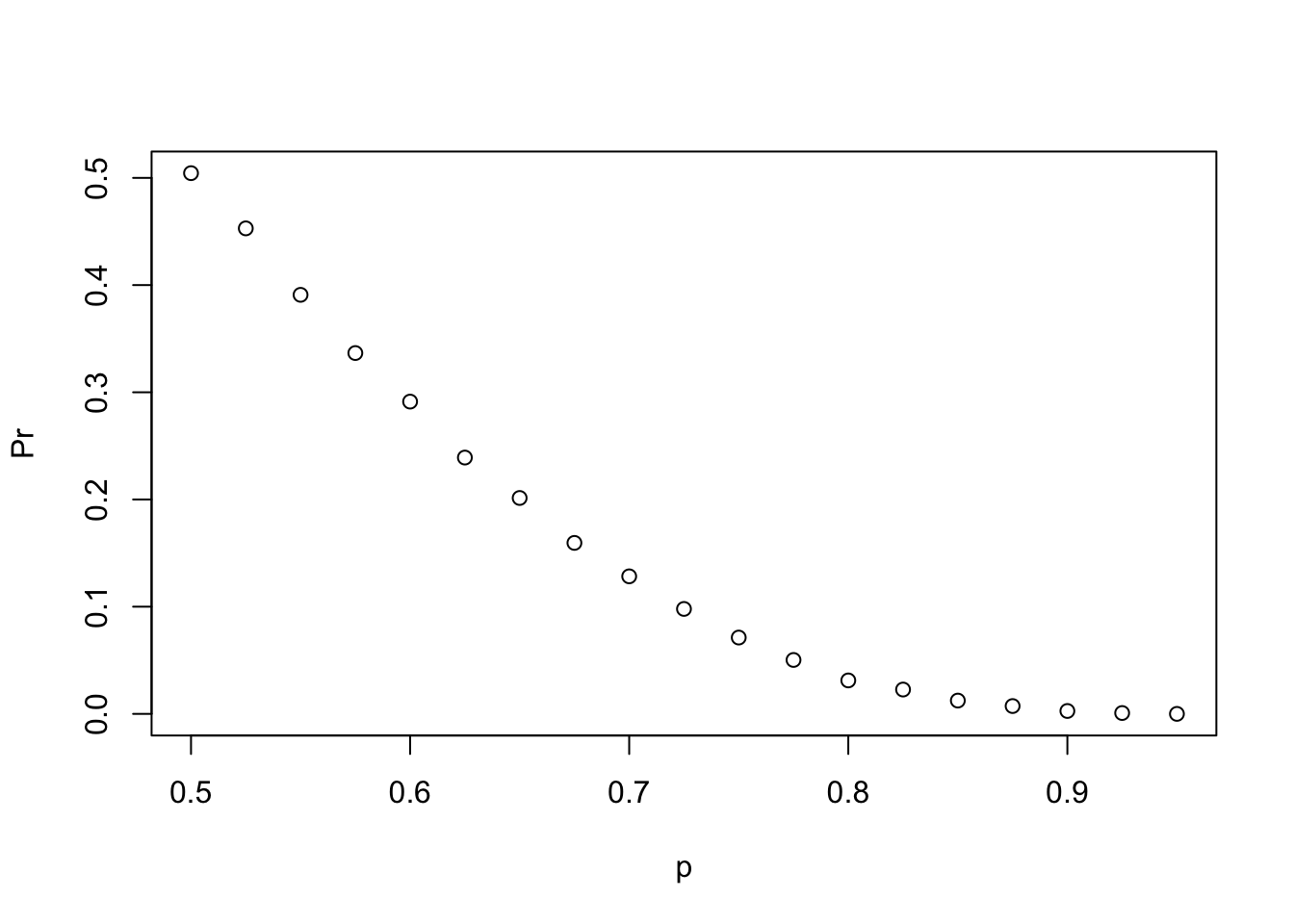
- Repeat the previous exercise, but now keep the probability that team \(A\) wins fixed at
p <- 0.75and compute the probability for different series lengths.
For example, wins in best of 1 game, 3 games, 5 games, and so on through a series that lasts 25 games.
# Given a value 'p', the probability of winning the series for the underdog team B can be computed with the following function based on a Monte Carlo simulation:
prob_win <- function(N, p=0.75){
      B <- 10000
      result <- replicate(B, {
        b_win <- sample(c(1,0), N, replace = TRUE, prob = c(1-p, p))
        sum(b_win)>=(N+1)/2
        })
      mean(result)
    }

# Assign the variable 'N' as the vector of series lengths. Use only odd numbers ranging from 1 to 25 games.
N <- seq(1, 25, 2)

# Apply the 'prob_win' function across the vector of series lengths to determine the probability that team B will win. Call this object `Pr`.
Pr <- sapply(N, prob_win)

# Plot the number of games in the series 'N' on the x-axis and 'Pr' on the y-axis.
plot(N,Pr)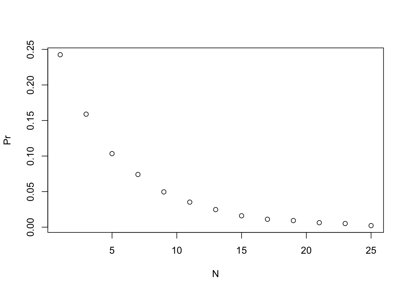
2.16 Assessment - Olympic Running
if(!require(tidyverse)) install.packages("tidyverse")## Loading required package: tidyverse## ── Attaching packages ───────────────────────────────────────────────────────────────────────────────────────────────────────────────────────────────────────────── tidyverse 1.3.0 ──## ✓ ggplot2 3.3.2 ✓ purrr 0.3.4
## ✓ tibble 3.0.3 ✓ dplyr 1.0.2
## ✓ tidyr 1.1.2 ✓ stringr 1.4.0
## ✓ readr 1.3.1 ✓ forcats 0.5.0## ── Conflicts ──────────────────────────────────────────────────────────────────────────────────────────────────────────────────────────────────────────────── tidyverse_conflicts() ──
## x dplyr::filter() masks stats::filter()
## x dplyr::lag() masks stats::lag()library(tidyverse)
options(digits = 3) # report 3 significant digits- In the 200m dash finals in the Olympics, 8 runners compete for 3 medals (order matters). In the 2012 Olympics, 3 of the 8 runners were from Jamaica and the other 5 were from different countries. The three medals were all won by Jamaica (Usain Bolt, Yohan Blake, and Warren Weir).
Use the information above to help you answer the following four questions.
1a. How many different ways can the 3 medals be distributed across 8 runners?
medals <- permutations(8,3)
nrow(medals)
## [1] 3361b. How many different ways can the three medals be distributed among the 3 runners from Jamaica?
jamaica <- permutations(3,3)
nrow(jamaica)
## [1] 61c. What is the probability that all 3 medals are won by Jamaica?
nrow(jamaica)/nrow(medals)## [1] 0.01791d. Run a Monte Carlo simulation on this vector representing the countries of the 8 runners in this race:
runners <- c("Jamaica", "Jamaica", "Jamaica", "USA", "Ecuador", "Netherlands", "France", "South Africa")For each iteration of the Monte Carlo simulation, within a replicate loop, select 3 runners representing the 3 medalists and check whether they are all from Jamaica. Repeat this simulation 10,000 times. Set the seed to 1 before running the loop.
Calculate the probability that all the runners are from Jamaica.
set.seed(1)
runners <- c("Jamaica", "Jamaica", "Jamaica", "USA", "Ecuador", "Netherlands", "France", "South Africa")
B <- 10000
all_jamaica <- replicate(B, {
  results <- sample(runners, 3)
  all(results == "Jamaica")
})
mean(all_jamaica)
## [1] 0.01742.17 Assessment - Restaurant Management
2: Use the information below to answer the following five questions.
A restaurant manager wants to advertise that his lunch special offers enough choices to eat different meals every day of the year. He doesn’t think his current special actually allows that number of choices, but wants to change his special if needed to allow at least 365 choices.
A meal at the restaurant includes 1 entree, 2 sides, and 1 drink. He currently offers a choice of 1 entree from a list of 6 options, a choice of 2 different sides from a list of 6 options, and a choice of 1 drink from a list of 2 options.
2a. How many meal combinations are possible with the current menu?
6 * nrow(combinations(6,2)) * 2## [1] 1802b. The manager has one additional drink he could add to the special.
How many combinations are possible if he expands his original special to 3 drink options?
6 * nrow(combinations(6,2)) * 3## [1] 2702c. The manager decides to add the third drink but needs to expand the number of options. The manager would prefer not to change his menu further and wants to know if he can meet his goal by letting customers choose more sides.
How many meal combinations are there if customers can choose from 6 entrees, 3 drinks, and select 3 sides from the current 6 options?
6 * nrow(combinations(6,3)) * 3## [1] 3602d. The manager is concerned that customers may not want 3 sides with their meal. He is willing to increase the number of entree choices instead, but if he adds too many expensive options it could eat into profits. He wants to know how many entree choices he would have to offer in order to meet his goal.
- Write a function that takes a number of entree choices and returns the number of meal combinations possible given that number of entree options, 3 drink choices, and a selection of 2 sides from 6 options.
- Use
sapplyto apply the function to entree option counts ranging from 1 to 12.
What is the minimum number of entree options required in order to generate more than 365 combinations?
entree_choices <- function(x){
  x * nrow(combinations(6,2)) * 3
}

combos <- sapply(1:12, entree_choices)

data.frame(entrees = 1:12, combos = combos) %>%
  filter(combos > 365) %>%
  min(.$entrees)
## [1] 92e. The manager isn’t sure he can afford to put that many entree choices on the lunch menu and thinks it would be cheaper for him to expand the number of sides. He wants to know how many sides he would have to offer to meet his goal of at least 365 combinations.
- Write a function that takes a number of side choices and returns the number of meal combinations possible given 6 entree choices, 3 drink choices, and a selection of 2 sides from the specified number of side choices.
- Use
sapplyto apply the function to side counts ranging from 2 to 12.
What is the minimum number of side options required in order to generate more than 365 combinations?
side_choices <- function(x){
  6 * nrow(combinations(x, 2)) * 3
}

combos <- sapply(2:12, side_choices)

data.frame(sides = 2:12, combos = combos) %>%
  filter(combos > 365) %>%
  min(.$sides)
## [1] 72.18 Assessment - Esophageal cancer and alcohol/tobacco use
3., 4., 5. and 6. Case-control studies help determine whether certain exposures are associated with outcomes such as developing cancer. The built-in dataset esoph contains data from a case-control study in France comparing people with esophageal cancer (cases, counted in ncases) to people without esophageal cancer (controls, counted in ncontrols) that are carefully matched on a variety of demographic and medical characteristics. The study compares alcohol intake in grams per day (alcgp) and tobacco intake in grams per day (tobgp) across cases and controls grouped by age range (agegp).
The dataset is available in base R and can be called with the variable name esoph:
head(esoph)## agegp alcgp tobgp ncases ncontrols
## 1 25-34 0-39g/day 0-9g/day 0 40
## 2 25-34 0-39g/day 10-19 0 10
## 3 25-34 0-39g/day 20-29 0 6
## 4 25-34 0-39g/day 30+ 0 5
## 5 25-34 40-79 0-9g/day 0 27
## 6 25-34 40-79 10-19 0 7You will be using this dataset to answer the following four multi-part questions (Questions 3-6).
You may wish to use the tidyverse package.
The following three parts have you explore some basic characteristics of the dataset.
Each row contains one group of the experiment. Each group has a different combination of age, alcohol consumption, and tobacco consumption. The number of cancer cases and number of controls (individuals without cancer) are reported for each group.
3a. How many groups are in the study?
nrow(esoph)## [1] 883b. How many cases are there?
Save this value as all_cases for later problems.
all_cases <- sum(esoph$ncases)
all_cases
## [1] 2003c. How many controls are there?
Save this value as all_controls for later problems. Remember from the instructions that controls are individuals without cancer.
all_controls <- sum(esoph$ncontrols)
all_controls
## [1] 9754a. What is the probability that a subject in the highest alcohol consumption group is a cancer case?
Remember that the total number of individuals in the study includes people with cancer (cases) and people without cancer (controls), so you must add both values together to get the denominator for your probability.
esoph %>%
  filter(alcgp == "120+") %>%
  summarize(ncases = sum(ncases), ncontrols = sum(ncontrols)) %>%
  mutate(p_case = ncases / (ncases + ncontrols)) %>%
  pull(p_case)
## [1] 0.4024b. What is the probability that a subject in the lowest alcohol consumption group is a cancer case?
esoph %>%
  filter(alcgp == "0-39g/day") %>%
  summarize(ncases = sum(ncases), ncontrols = sum(ncontrols)) %>%
  mutate(p_case = ncases / (ncases + ncontrols)) %>%
  pull(p_case)
## [1] 0.06534c. Given that a person is a case, what is the probability that they smoke 10g or more a day?
tob_cases <- esoph %>%
  filter(tobgp != "0-9g/day") %>%
  pull(ncases) %>%
  sum()

tob_cases/all_cases
## [1] 0.614d. Given that a person is a control, what is the probability that they smoke 10g or more a day?
tob_controls <- esoph %>%
  filter(tobgp != "0-9g/day") %>%
  pull(ncontrols) %>%
  sum()

tob_controls/all_controls
## [1] 0.4625a. For cases, what is the probability of being in the highest alcohol group?
high_alc_cases <- esoph %>%
  filter(alcgp == "120+") %>%
  pull(ncases) %>%
  sum()

p_case_high_alc <- high_alc_cases/all_cases
p_case_high_alc
## [1] 0.2255b. For cases, what is the probability of being in the highest tobacco group?
high_tob_cases <- esoph %>%
  filter(tobgp == "30+") %>%
  pull(ncases) %>%
  sum()

p_case_high_tob <- high_tob_cases/all_cases
p_case_high_tob
## [1] 0.1555c. For cases, what is the probability of being in the highest alcohol group and the highest tobacco group?
high_alc_tob_cases <- esoph %>%
  filter(alcgp == "120+" & tobgp == "30+") %>%
  pull(ncases) %>%
  sum()

p_case_high_alc_tob <- high_alc_tob_cases/all_cases
p_case_high_alc_tob
## [1] 0.055d. For cases, what is the probability of being in the highest alcohol group or the highest tobacco group?
p_case_either_highest <- p_case_high_alc + p_case_high_tob - p_case_high_alc_tob
p_case_either_highest
## [1] 0.336a. For controls, what is the probability of being in the highest alcohol group?
high_alc_controls <- esoph %>%
  filter(alcgp == "120+") %>%
  pull(ncontrols) %>%
  sum()

p_control_high_alc <- high_alc_controls/all_controls
p_control_high_alc
## [1] 0.06876b. How many times more likely are cases than controls to be in the highest alcohol group?
p_case_high_alc/p_control_high_alc## [1] 3.276c. For controls, what is the probability of being in the highest tobacco group?
high_tob_controls <- esoph %>%
  filter(tobgp == "30+") %>%
  pull(ncontrols) %>%
  sum()

p_control_high_tob <- high_tob_controls/all_controls
p_control_high_tob
## [1] 0.08416d. For controls, what is the probability of being in the highest alcohol group and the highest tobacco group?
high_alc_tob_controls <- esoph %>%
  filter(alcgp == "120+" & tobgp == "30+") %>%
  pull(ncontrols) %>%
  sum()

p_control_high_alc_tob <- high_alc_tob_controls/all_controls
p_control_high_alc_tob
## [1] 0.01336e. For controls, what is the probability of being in the highest alcohol group or the highest tobacco group?
p_control_either_highest <- p_control_high_alc + p_control_high_tob - p_control_high_alc_tob
p_control_either_highest
## [1] 0.1396f. How many times more likely are cases than controls to be in the highest alcohol group or the highest tobacco group?
p_case_either_highest/p_control_either_highest## [1] 2.37