3 Section 2 Overview
Section 2 introduces you to Continuous Probability.
After completing Section 2, you will:
- understand the differences between calculating probabilities for discrete and continuous data.
- be able to use cumulative distribution functions to assign probabilities to intervals when dealing with continuous data.
- be able to use R to generate normally distributed outcomes for use in Monte Carlo simulations.
- know some of the useful theoretical continuous distributions in addition to the normal distribution, such as the student-t, chi-squared, exponential, gamma, beta, and beta-binomial distributions.
3.1 Continuous Probability
The textbook for this section is available here.
The previous discussion of CDF is from the Data Visualization course. Here is the textbook section on the CDF.
Key points
- The cumulative distribution function (CDF) is a distribution function for continuous data \(x\) that reports the proportion of the data below \(a\) for all values of \(a\):
\(F(a) = \mbox{Pr}(a) = \mbox{Pr}(x \le a)\)
- The CDF is the probability distribution function for continuous variables. For example, to determine the probability that a male student is taller than 70.5 inches given a vector of male heights \(x\), we can use the CDF:
\(\mbox{Pr}(x > 70.5) = 1 − \mbox{Pr}(x \le 70.5) = 1 − F(70.5)\)
- The probability that an observation is in between two values \(a, b\) is \(F(b) - F(a)\).
Code: Cumulative distribution function
Define x as male heights from the dslabs dataset:
if(!require(dslabs)) install.packages("dslabs")## Loading required package: dslabslibrary(dslabs)
data(heights)
x <- heights %>% filter(sex=="Male") %>% pull(height)Given a vector x, we can define a function for computing the CDF of x using:
F <- function(a) mean(x <= a)
1 - F(70) # probability of male taller than 70 inches## [1] 0.3773.2 Theoretical Distribution
The textbook for this section is available here.
Key points
- pnorm(a, avg, s) gives the value of the cumulative distribution function \(F(a)\) for the normal distribution defined by average avg and standard deviation s.
- We say that a random quantity is normally distributed with average avg and standard deviation s if the approximation pnorm(a, avg, s) holds for all values of a.
- If we are willing to use the normal approximation for height, we can estimate the distribution simply from the mean and standard deviation of our values.
- If we treat the height data as discrete rather than categorical, we see that the data are not very useful because integer values are more common than expected due to rounding. This is called discretization.
- With rounded data, the normal approximation is particularly useful when computing probabilities of intervals of length 1 that include exactly one integer.
Code: Using pnorm to calculate probabilities
Given male heights x:
x <- heights %>% filter(sex=="Male") %>% pull(height)We can estimate the probability that a male is taller than 70.5 inches using:
1 - pnorm(70.5, mean(x), sd(x))## [1] 0.371Code: Discretization and the normal approximation
# plot distribution of exact heights in data
plot(prop.table(table(x)), xlab = "a = Height in inches", ylab = "Pr(x = a)")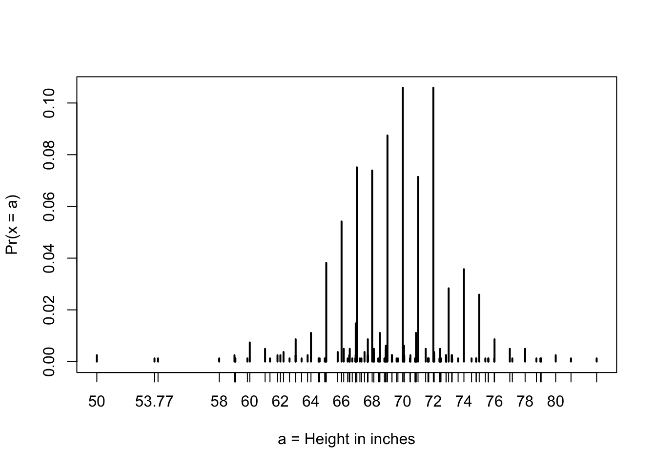
# probabilities in actual data over length 1 ranges containing an integer
mean(x <= 68.5) - mean(x <= 67.5)## [1] 0.115mean(x <= 69.5) - mean(x <= 68.5)## [1] 0.119mean(x <= 70.5) - mean(x <= 69.5)## [1] 0.122# probabilities in normal approximation match well
pnorm(68.5, mean(x), sd(x)) - pnorm(67.5, mean(x), sd(x))## [1] 0.103pnorm(69.5, mean(x), sd(x)) - pnorm(68.5, mean(x), sd(x))## [1] 0.11pnorm(70.5, mean(x), sd(x)) - pnorm(69.5, mean(x), sd(x))## [1] 0.108# probabilities in actual data over other ranges don't match normal approx as well
mean(x <= 70.9) - mean(x <= 70.1)## [1] 0.0222pnorm(70.9, mean(x), sd(x)) - pnorm(70.1, mean(x), sd(x))## [1] 0.08363.3 Probability Density
The textbook for this section is available here.
Key points
- The probability of a single value is not defined for a continuous distribution.
- The quantity with the most similar interpretation to the probability of a single value is the probability density function \(f(x)\).
- The probability density \(f(x)\) is defined such that the integral of \(f(x)\) over a range gives the CDF of that range.
\(F(a) = \mbox{Pr}(X \le a) = \int_{-\infty}^{a} f(x)dx\)
- In R, the probability density function for the normal distribution is given by dnorm. We will see uses of dnorm in the future.
- Note that dnorm gives the density function and pnorm gives the distribution function, which is the integral of the density function.
3.4 Monte Carlo simulations
The textbook for this section is available here.
Key points
- rnorm(n, avg, s) generates n random numbers from the normal distribution with average avg and standard deviation s.
- By generating random numbers from the normal distribution, we can simulate height data with similar properties to our dataset. Here we generate simulated height data using the normal distribution.
Code: Generating normally distributed random numbers for Monte Carlo simulations
# define x as male heights from dslabs data
library(tidyverse)
library(dslabs)
data(heights)
x <- heights %>% filter(sex=="Male") %>% pull(height)
# generate simulated height data using normal distribution - both datasets should have n observations
n <- length(x)
avg <- mean(x)
s <- sd(x)
simulated_heights <- rnorm(n, avg, s)
# plot distribution of simulated_heights
data.frame(simulated_heights = simulated_heights) %>%
ggplot(aes(simulated_heights)) +
geom_histogram(color="black", binwidth = 2)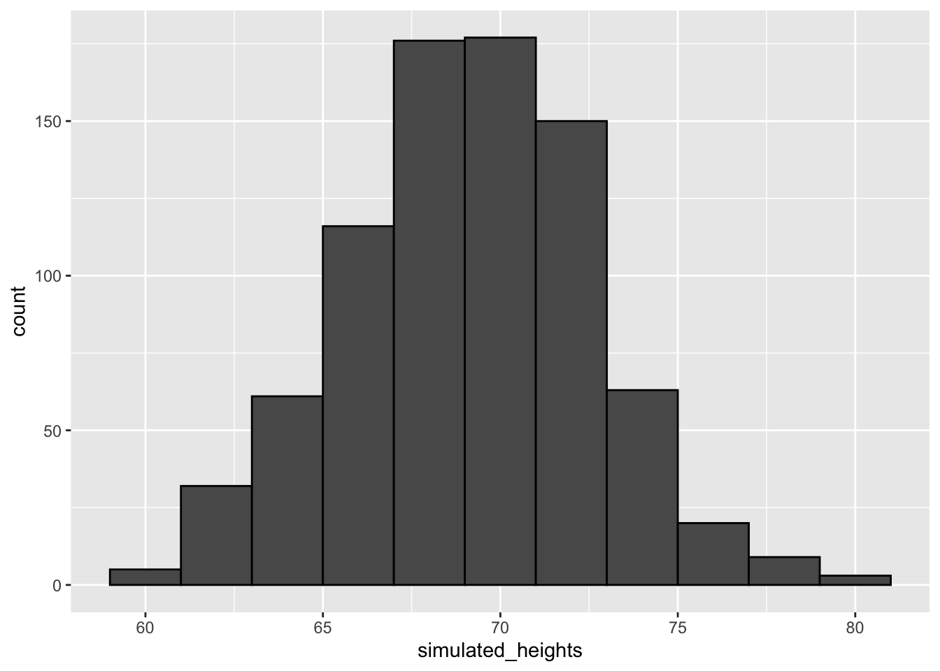
Code: Monte Carlo simulation of probability of tallest person being over 7 feet
B <- 10000
tallest <- replicate(B, {
    simulated_data <- rnorm(800, avg, s)    # generate 800 normally distributed random heights
    max(simulated_data)    # determine the tallest height
})
mean(tallest >= 7*12)    # proportion of times that tallest person exceeded 7 feet (84 inches)
## [1] 0.02093.5 Other Continuous Distributions
The textbook for this section is available here.
Key points
- You may encounter other continuous distributions (Student t, chi-squared, exponential, gamma, beta, etc.).
- R provides functions for density (d), quantile (q), probability distribution (p) and random number generation (r) for many of these distributions.
- Each distribution has a matching abbreviation (for example, norm or t) that is paired with the related function abbreviations (d, p, q, r) to create appropriate functions.
- For example, use rt to generate random numbers for a Monte Carlo simulation using the Student t distribution.
Code: Plotting the normal distribution with dnorm
Use d to plot the density function of a continuous distribution. Here is the density function for the normal distribution (abbreviation norm):
x <- seq(-4, 4, length.out = 100)
data.frame(x, f = dnorm(x)) %>%
    ggplot(aes(x,f)) +
    geom_line()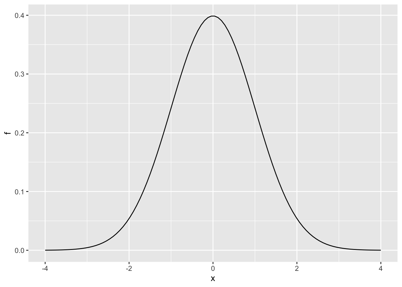
3.6 Assessment - Continuous Probability
- Assume the distribution of female heights is approximated by a normal distribution with a mean of 64 inches and a standard deviation of 3 inches.
If we pick a female at random, what is the probability that she is 5 feet or shorter?
# Assign a variable 'female_avg' as the average female height.
female_avg <- 64

# Assign a variable 'female_sd' as the standard deviation for female heights.
female_sd <- 3

# Using variables 'female_avg' and 'female_sd', calculate the probability that a randomly selected female is shorter than 5 feet. Print this value to the console.
pnorm((5*12), female_avg, female_sd)
## [1] 0.0912- Assume the distribution of female heights is approximated by a normal distribution with a mean of 64 inches and a standard deviation of 3 inches.
If we pick a female at random, what is the probability that she is 6 feet or taller?
# Assign a variable 'female_avg' as the average female height.
female_avg <- 64

# Assign a variable 'female_sd' as the standard deviation for female heights.
female_sd <- 3

# Using variables 'female_avg' and 'female_sd', calculate the probability that a randomly selected female is 6 feet or taller. Print this value to the console.
1-pnorm((6*12), female_avg, female_sd)
## [1] 0.00383- Assume the distribution of female heights is approximated by a normal distribution with a mean of 64 inches and a standard deviation of 3 inches.
If we pick a female at random, what is the probability that she is between 61 and 67 inches?
# Assign a variable 'female_avg' as the average female height.
female_avg <- 64

# Assign a variable 'female_sd' as the standard deviation for female heights.
female_sd <- 3

# Using variables 'female_avg' and 'female_sd', calculate the probability that a randomly selected female is between the desired height range. Print this value to the console.
pnorm(67, female_avg, female_sd) - pnorm(61, female_avg, female_sd)
## [1] 0.683- Repeat the previous exercise, but convert everything to centimeters.
That is, multiply every height, including the standard deviation, by 2.54. What is the answer now?
# Assign a variable 'female_avg' as the average female height. Convert this value to centimeters.
female_avg <- 64*2.54

# Assign a variable 'female_sd' as the standard deviation for female heights. Convert this value to centimeters.
female_sd <- 3*2.54

# Using variables 'female_avg' and 'female_sd', calculate the probability that a randomly selected female is between the desired height range. Print this value to the console.
pnorm((67*2.54), female_avg, female_sd) - pnorm((61*2.54), female_avg, female_sd)
## [1] 0.683- Compute the probability that the height of a randomly chosen female is within 1 SD from the average height.
# Assign a variable 'female_avg' as the average female height.
female_avg <- 64

# Assign a variable 'female_sd' as the standard deviation for female heights.
female_sd <- 3

# To a variable named 'taller', assign the value of a height that is one SD taller than average.
taller <- female_avg + female_sd

# To a variable named 'shorter', assign the value of a height that is one SD shorter than average.
shorter <- female_avg - female_sd

# Calculate the probability that a randomly selected female is between the desired height range. Print this value to the console.
pnorm(taller, female_avg, female_sd) - pnorm(shorter, female_avg, female_sd)
## [1] 0.683- Imagine the distribution of male adults is approximately normal with an expected value of 69 inches and a standard deviation of 3 inches.
How tall is a male in the 99th percentile?
# Assign a variable 'male_avg' as the average male height.
male_avg <- 69

# Assign a variable 'male_sd' as the standard deviation for male heights.
male_sd <- 3

# Determine the height of a man in the 99th percentile of the distribution.
qnorm(0.99, male_avg, male_sd)
## [1] 76- The distribution of IQ scores is approximately normally distributed.
The average is 100 and the standard deviation is 15. Suppose you want to know the distribution of the person with the highest IQ in your school district, where 10,000 people are born each year.
Generate 10,000 IQ scores 1,000 times using a Monte Carlo simulation. Make a histogram of the highest IQ scores.
# The variable `B` specifies the number of times we want the simulation to run.
B <- 1000

# Use the `set.seed` function to make sure your answer matches the expected result after random number generation.
set.seed(1)

# Create an object called `highestIQ` that contains the highest IQ score from each random distribution of 10,000 people.
highestIQ <- replicate(B, {
    IQ <- rnorm(10000, 100, 15)
    max(IQ)
})

# Make a histogram of the highest IQ scores.
hist(highestIQ)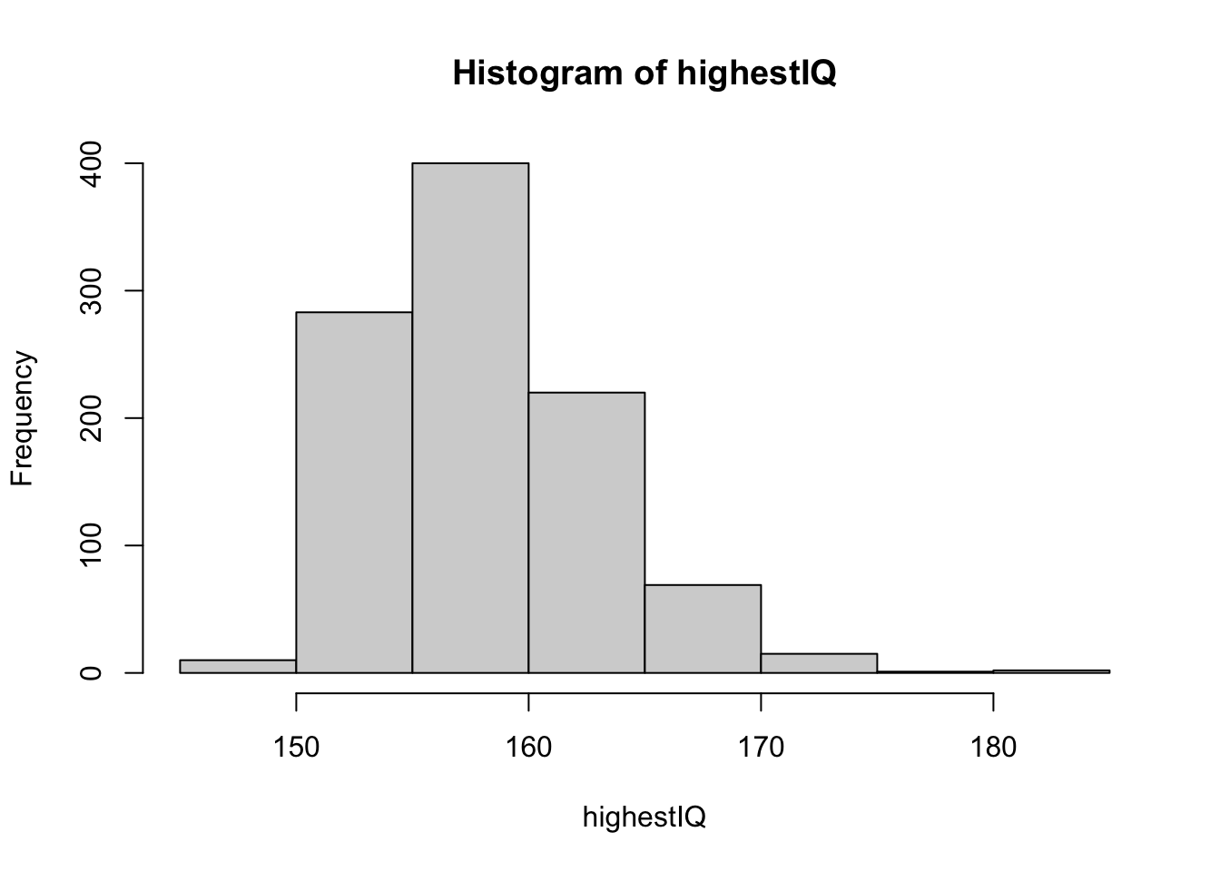
3.7 Assessment - ACT scores, part 1
- and 2. The ACT is a standardized college admissions test used in the United States. The four multi-part questions in this assessment all involve simulating some ACT test scores and answering probability questions about them.
For the three year period 2016-2018, ACT standardized test scores were approximately normally distributed with a mean of 20.9 and standard deviation of 5.7. (Real ACT scores are integers between 1 and 36, but we will ignore this detail and use continuous values instead.)
First we’ll simulate an ACT test score dataset and answer some questions about it.
Set the seed to 16, then use rnorm to generate a normal distribution of 10000 tests with a mean of 20.9 and standard deviation of 5.7. Save these values as act_scores. You’ll be using this dataset throughout these four multi-part questions.
(IMPORTANT NOTE! If you use R 3.6 or later, you will need to use the command set.seed(x, sample.kind = “Rounding”) instead of set.seed(x). Your R version will be printed at the top of the Console window when you start RStudio.)
1a. What is the mean of act_scores?
set.seed(16, sample.kind = "Rounding")## Warning in set.seed(16, sample.kind = "Rounding"): non-uniform 'Rounding' sampler usedact_scores <- rnorm(10000, 20.9, 5.7)
mean(act_scores)## [1] 20.81b. What is the standard deviation of act_scores?
sd(act_scores)## [1] 5.681c. A perfect score is 36 or greater (the maximum reported score is 36).
In act_scores, how many perfect scores are there out of 10,000 simulated tests?
sum(act_scores >= 36)## [1] 411d. In act_scores, what is the probability of an ACT score greater than 30?
mean(act_scores > 30)## [1] 0.05271e. In act_scores, what is the probability of an ACT score less than or equal to 10?
mean(act_scores <= 10)## [1] 0.0282- Set
xequal to the sequence of integers 1 to 36. Usednormto determine the value of the probability density function overxgiven a mean of 20.9 and standard deviation of 5.7; save the result asf_x. Plotxagainstf_x.
x <- 1:36
f_x <- dnorm(x, 20.9, 5.7)
data.frame(x, f_x) %>%
  ggplot(aes(x, f_x)) +
  geom_line()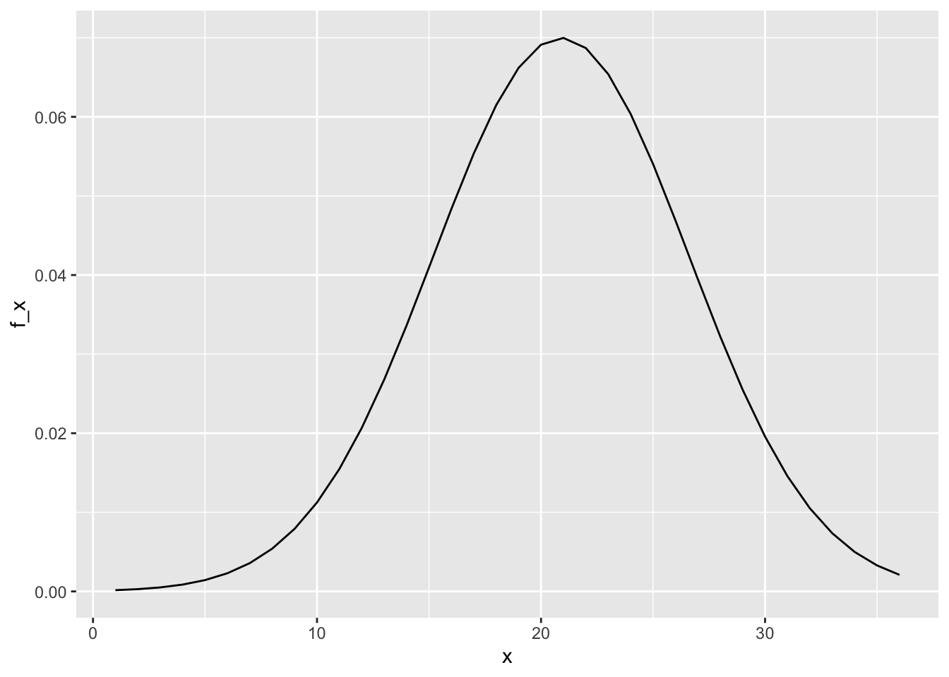
Which of the following plots is correct?
- B.
Plot x against f_x
3.8 Assessment - ACT scores, part 2
- In this 3-part question, you will convert raw ACT scores to Z-scores and answer some questions about them.
Convert act_scores to Z-scores. Recall from Data Visualization (the second course in this series) that to standardize values (convert values into Z-scores, that is, values distributed with a mean of 0 and standard deviation of 1), you must subtract the mean and then divide by the standard deviation. Use the mean and standard deviation of act_scores, not the original values used to generate random test scores.
3a. What is the probability of a Z-score greater than 2 (2 standard deviations above the mean)?
z_scores <- (act_scores - mean(act_scores))/sd(act_scores)
mean(z_scores > 2)
## [1] 0.02333b. What ACT score value corresponds to 2 standard deviations above the mean (Z = 2)?
2*sd(act_scores) + mean(act_scores)## [1] 32.23c. A Z-score of 2 corresponds roughly to the 97.5th percentile.
Use qnorm to determine the 97.5th percentile of normally distributed data with the mean and standard deviation observed in act_scores.
What is the 97.5th percentile of act_scores?
qnorm(.975, mean(act_scores), sd(act_scores))## [1] 32- In this 4-part question, you will write a function to create a CDF for ACT scores.
Write a function that takes a value and produces the probability of an ACT score less than or equal to that value (the CDF). Apply this function to the range 1 to 36.
4a. What is the minimum integer score such that the probability of that score or lower is at least .95?
Your answer should be an integer 1-36.
cdf <- sapply(1:36, function (x){
  mean(act_scores <= x)
})
min(which(cdf >= .95))
## [1] 314b. Use qnorm to determine the expected 95th percentile, the value for which the probability of receiving that score or lower is 0.95, given a mean score of 20.9 and standard deviation of 5.7.
What is the expected 95th percentile of ACT scores?
qnorm(.95, 20.9, 5.7)## [1] 30.34c. As discussed in the Data Visualization course, we can use quantile to determine sample quantiles from the data.
Make a vector containing the quantiles for p <- seq(0.01, 0.99, 0.01), the 1st through 99th percentiles of the act_scores data. Save these as sample_quantiles.
In what percentile is a score of 26?
Note that a score between the 98th and 99th percentile should be considered the 98th percentile, for example, and that quantile numbers are used as names for the vector sample_quantiles.
p <- seq(0.01, 0.99, 0.01)
sample_quantiles <- quantile(act_scores, p)
names(sample_quantiles[max(which(sample_quantiles < 26))])
## [1] "82%"4d. Make a corresponding set of theoretical quantiles using qnorm over the interval p <- seq(0.01, 0.99, 0.01) with mean 20.9 and standard deviation 5.7. Save these as theoretical_quantiles. Make a QQ-plot graphing sample_quantiles on the y-axis versus theoretical_quantiles on the x-axis.
p <- seq(0.01, 0.99, 0.01)
sample_quantiles <- quantile(act_scores, p)
theoretical_quantiles <- qnorm(p, 20.9, 5.7)
qplot(theoretical_quantiles, sample_quantiles) + geom_abline()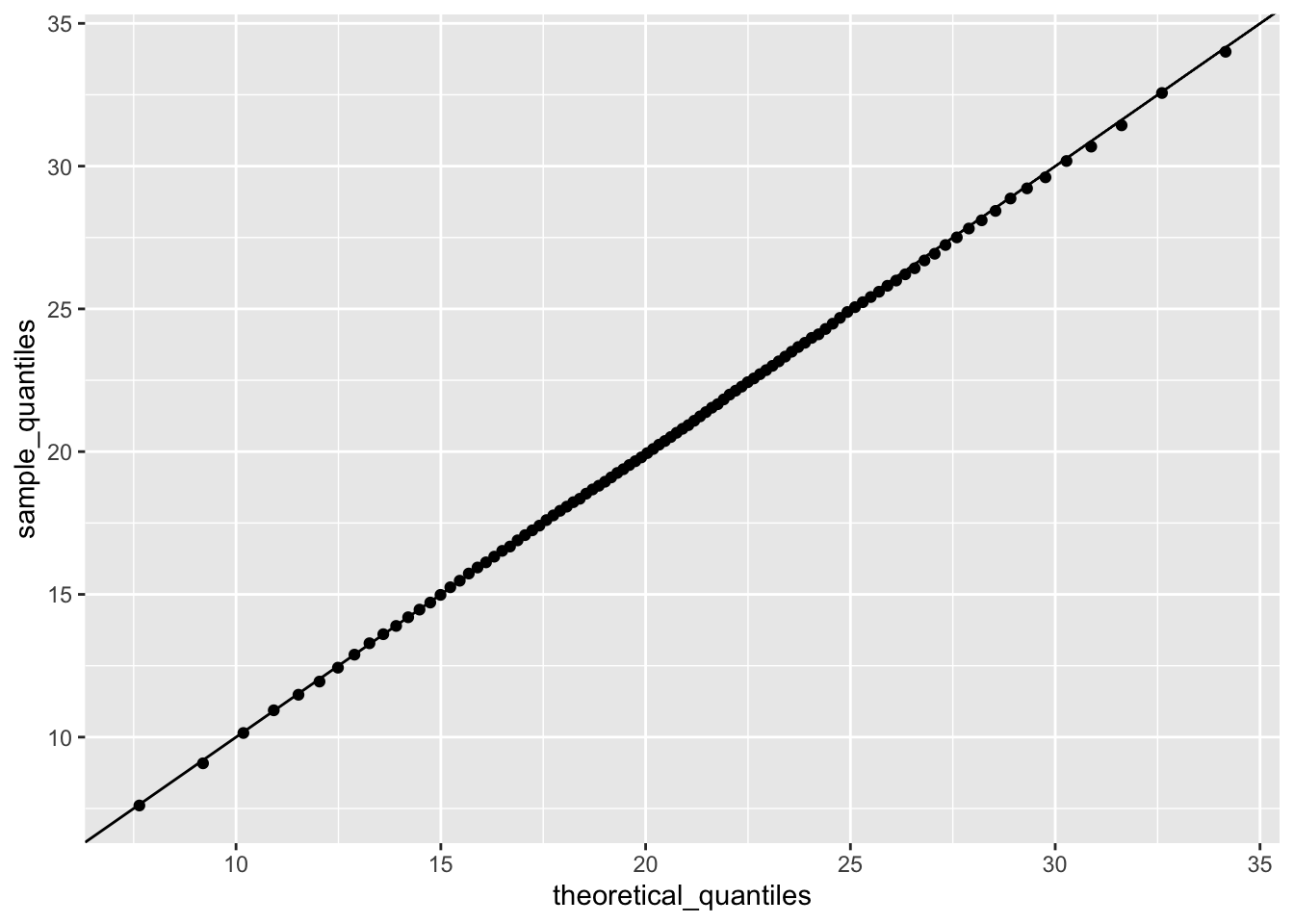
Which of the following graphs is correct?
- D.
Sample quantiles versus Theoretical quantiles